|
|
|
|
Simulating propagation of separated wave modes in general anisotropic media, Part II: qS-wave propagators |
For comparison, we first apply the original elastic wave equation
to synthesize wavefields in a homogeneous VTI medium with weak anisotropy, in which
![]() ,
,
![]() ,
,
![]() , and
, and
![]() .
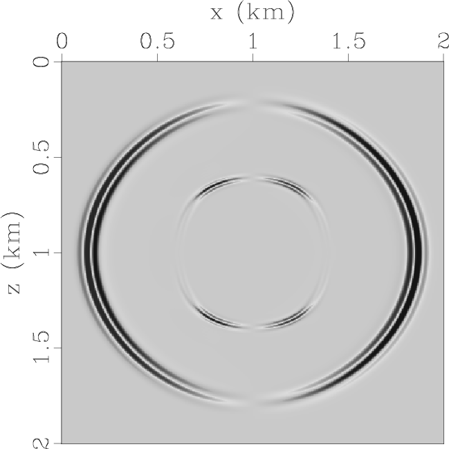
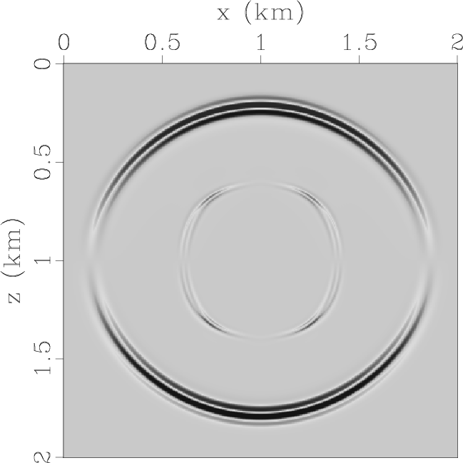
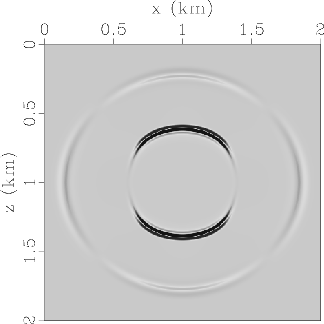
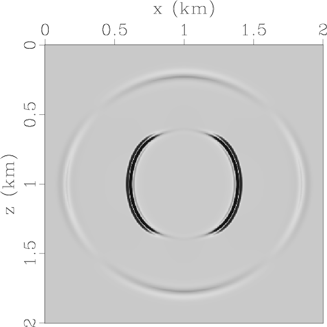
Figures 2a and 2b display the horizontal and vertical components of the displacement
wavefields at 0.3 s.
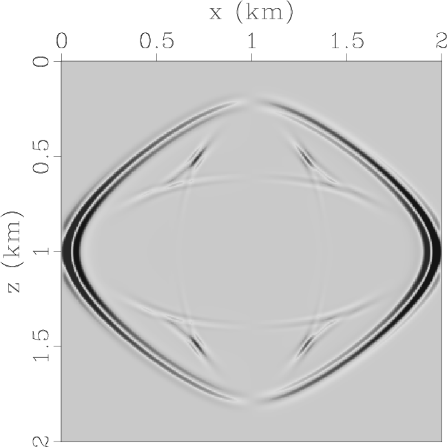
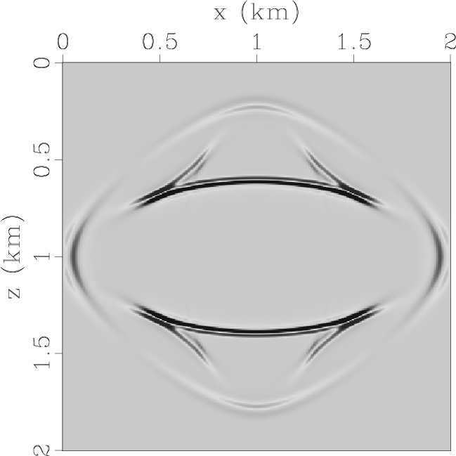
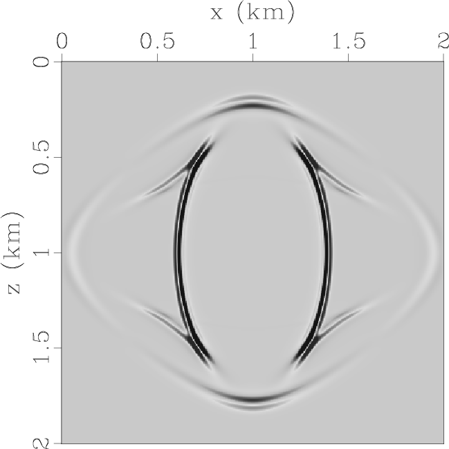
Then we try to simulate the propagation of a single-mode qSV-wave using the pseudo-pure-mode qSV-wave equation
(namely equation 30).
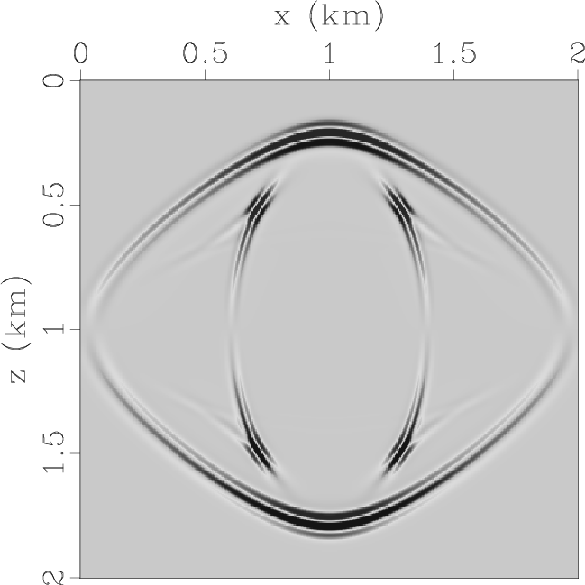
Figure 2c and 2d display the two components of the pseudo-pure-mode qSV-wave fields,
and Figure 2e displays their summation, i.e., the pseudo-pure-mode scalar qSV-wave
fields with weak residual qP-wave energy.
We observe that, in most propagation directions, the polarities are almost reversed for the wavefronts of qP-waves
in the two components of the pseudo-pure-mode qSV-wave fields.
This contributes to suppressing the qP-wave energy through summation of the two components.
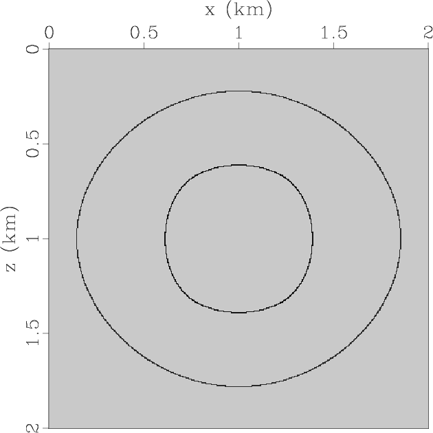
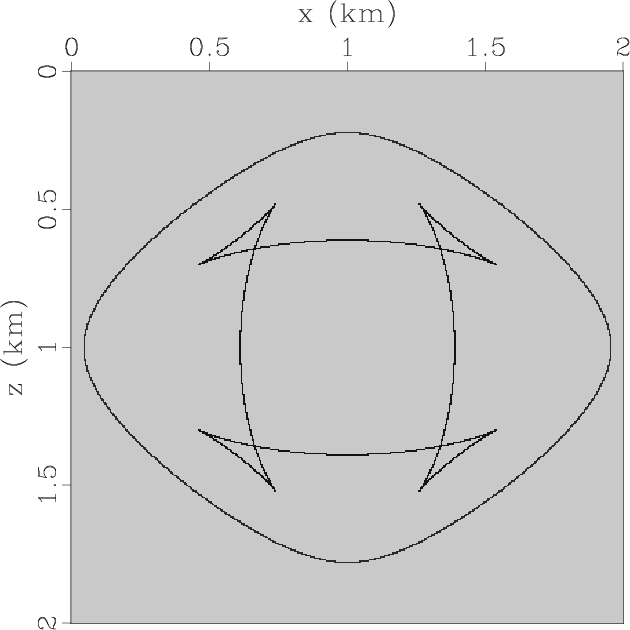
Compared with the theoretical wavefront curves (see Figure 2f) calculated
using group velocities
and angles, pseudo-pure-mode scalar qSV-wave fields have correct kinematics for
both qP- and qSV-waves.
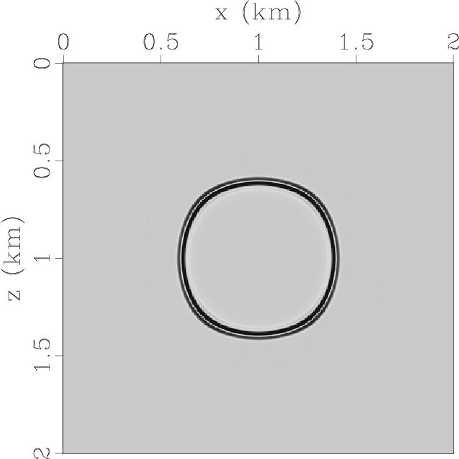
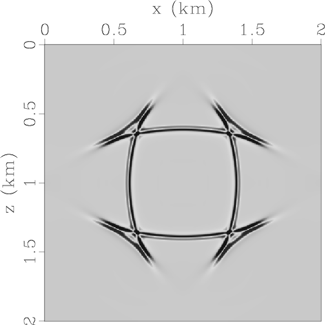
We finally remove residual qP-waves by applying the filtering to correct the projection deviation
and get completely separated scalar qSV-wave fields (Figure 2g).
.
Figures 2a and 2b display the horizontal and vertical components of the displacement
wavefields at 0.3 s.
Then we try to simulate the propagation of a single-mode qSV-wave using the pseudo-pure-mode qSV-wave equation
(namely equation 30).
Figure 2c and 2d display the two components of the pseudo-pure-mode qSV-wave fields,
and Figure 2e displays their summation, i.e., the pseudo-pure-mode scalar qSV-wave
fields with weak residual qP-wave energy.
We observe that, in most propagation directions, the polarities are almost reversed for the wavefronts of qP-waves
in the two components of the pseudo-pure-mode qSV-wave fields.
This contributes to suppressing the qP-wave energy through summation of the two components.
Compared with the theoretical wavefront curves (see Figure 2f) calculated
using group velocities
and angles, pseudo-pure-mode scalar qSV-wave fields have correct kinematics for
both qP- and qSV-waves.
We finally remove residual qP-waves by applying the filtering to correct the projection deviation
and get completely separated scalar qSV-wave fields (Figure 2g).

|
|---|
|
Elasticx,Elasticz,PseudoPureSVx,PseudoPureSVz,PseudoPureSV,WF,PseudoPureSepSV
Figure 2. Synthesized wavefields in a VTI medium with weak anisotropy: (a) x- and (b) z-components synthesized by original elastic wave equation; (c) x- and (d) z-components synthesized by pseudo-pure-mode qSV-wave equation; (e) pseudo-pure-mode scalar qSV-wave fields; (f) kinematics of qV- and qSV-waves and (g) separated scalar qSV-wave fields. |
|
|
Next, we consider wavefield modeling in a homogeneous VTI medium with strong
anisotropy,
in which
![]() ,
,
![]() ,
,
![]() , and
, and
![]() .
Figure 3 displays the wavefield snapshots at 0.3 s synthesized both by using the original
elastic wave equation
and the pseudo-pure-mode qSV-wave equation. Note that the pseudo-pure-mode
qSV-wave equation still accurately
represents the qP- and qSV-waves' kinematics. Although the residual qP-wave energy
becomes stronger when
the degree of anisotropy increases, the filtering step still removes them effectively.
It takes CPU times of 0.15 and 0.06 seconds to extrapolate the elastic and pseudo-pure-mode qSV-wave fields for one time-step, respectively.
But it takes about 8.2 seconds to remove the residual qP-wave from the pseudo-pure-mode qSV-wave fields using wavenumber-domain filtering.
In fact, separating the pure-mode wavefield from the elastic and pseudo-pure-mode wavefields has almost the same computational cost for TI media (Cheng and Kang, 2014).
.
Figure 3 displays the wavefield snapshots at 0.3 s synthesized both by using the original
elastic wave equation
and the pseudo-pure-mode qSV-wave equation. Note that the pseudo-pure-mode
qSV-wave equation still accurately
represents the qP- and qSV-waves' kinematics. Although the residual qP-wave energy
becomes stronger when
the degree of anisotropy increases, the filtering step still removes them effectively.
It takes CPU times of 0.15 and 0.06 seconds to extrapolate the elastic and pseudo-pure-mode qSV-wave fields for one time-step, respectively.
But it takes about 8.2 seconds to remove the residual qP-wave from the pseudo-pure-mode qSV-wave fields using wavenumber-domain filtering.
In fact, separating the pure-mode wavefield from the elastic and pseudo-pure-mode wavefields has almost the same computational cost for TI media (Cheng and Kang, 2014).

|
|---|
|
Elasticx,Elasticz,PseudoPureSVx,PseudoPureSVz,PseudoPureSV,WF,PseudoPureSepSV
Figure 3. The same plots as Figure 2 but for a VTI medium with stronger anisotropy. |
|
|
|
|
|
|
Simulating propagation of separated wave modes in general anisotropic media, Part II: qS-wave propagators |