Simulating propagation of separated wave modes in general anisotropic media, Part I: qP-wave propagators

Pseudo-pure-mode qP-wave equation in VTI media

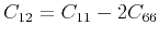
For a VTI medium, there are only five independent parameters: $C_{11}$ , $C_{33}$ , $C_{44}$ , $C_{66}$ and $C_{13}$ , with $C_{12}=C_{11}-2C_{66}$ , $C_{22}=C_{11}$ , $C_{23}=C_{13}$ and $C_{55}=C_{44}$ . So we rewrite equation 18 as,

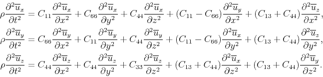$$\begin{split}\rho\frac{\partial^2{\overline{u}_x}}{\partial t... ...4})\frac{\partial^2{\overline{u}_y}}{\partial z^2}. \end{split}$$ (19)

Since a TI material has cylindrical symmetry in its elastic properties, it is safe to sum the first two equations in equation 19 to yield a simplified form for wavefield modeling and RTM, namely

$$\begin{split}\rho\frac{\partial^2{\overline{u}_{xy}}}{\partia... ...\frac{\partial^2{\overline{u}_{xy}}}{\partial z^2}, \end{split}$$ (20)

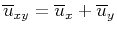where $\overline{u}_{xy}=\overline{u}_{x}+\overline{u}_{y}$ represents the sum of the two horizontal components. Pure SH-waves horizontally polarize in the isotropic planes of VTI media with the polarization given by $(-k_{y}, k_{x}, 0)$ , which implies $ik_{x}\widetilde{u}_{x}+ik_{y}\widetilde{u}_{y}=0$ , i.e., $\overline{u}_{xy}=0$ , for the SH-wave. Therefore, the above partial summation (after the first-step projection) completes divergence operation and removes the SH-waves from the three-component pseudo-pure-mode qP-wave fields. As a result, there are no terms related to $C_{66}$ any more in equation 20. Compared with original elastic wave equation, equation 20 further reduces the compuational costs for 3D wavefield modeling and RTM for VTI media.

Applying the Thomsen notation (Thomsen, 1986),

$$\begin{split}C_{11} &= (1+2\epsilon)\rho{v_{p0}^2}, C_{33}... ...ho^2({v_{p0}^2}-{v_{s0}^2})({v_{pn}^2}-{v_{s0}^2}), \end{split}$$ (21)

the pseudo-pure-mode qP-wave equation can be expressed as,

$$\begin{split}\frac{\partial^2\overline{u}_{xy}}{\partial t^2}... ...} \frac{\partial^2\overline{u}_{xy}}{\partial z^2}, \end{split}$$ (22)

where $v_{p0}$ and $v_{s0}$ represent the vertical velocities of qP- and qSV-waves, $v_{pn} = v_{p0}\sqrt{1+2\delta}$ represents the interval NMO velocity, $v_{px} = v_{p0}\sqrt{1+2\epsilon}$ represents the horizontal velocity of qP-waves, $\delta$ and $\epsilon$ are the other two Thomsen coefficients. Unlike other coupled second-order systems derived from the dispersion relation of VTI media (Zhou et al., 2006b), the wavefield components in equations 20 and 22 have clear physical meaning and their summation automatically produces scalar wavefields dominant of qP-wave energy. Equation 22 is also similar to a minimal coupled system (equation 30 in their paper) demonstrated by Fowler et al. (2010), except that it is now derived from a significant similarity transformation that helps to enhance qP-waves and suppress qS-waves (after summing the transformed wavefield components). This is undoubtedly useful for migration of conventional seismic data representing mainly qP-wave data.

We can also obtain a pseudo-acoustic coupled system by setting $v_{s0}=0$ in equation 22, namely:

$$\begin{split}\frac{\partial^2\overline{u}_{xy}}{\partial t^2}... ...2}\frac{\partial^2\overline{u}_{xy}}{\partial z^2}. \end{split}$$ (23)

The pseudo-acoustic approximation does not significantly affect the kinematic signatures but may distort the reflection, transmission and conversion coefficients (thus the amplitudes) of waves in elastic media.

If we further apply the isotropic assumption (seting $\delta=0$ and $\epsilon=0$ ) and sum the two equations in equation 23, we get the familar constant-density acoustic wave equation:

$$\frac{\partial^2\overline{u}}{\partial t^2} = {v_{p}^2}(\frac{\pa... ...\frac{\partial^2}{\partial y^2}+\frac{\partial^2}{\partial z^2}){\overline{u}},$$ (24)

where $\overline{u}=\overline{u}_{xy}+\overline{u}_{z}$ represents the acoustic pressure wavefield, and $v_{p}$ is the propagation velocity of isotropic P-wave.

Simulating propagation of separated wave modes in general anisotropic media, Part I: qP-wave propagators