next up previous [pdf]

Next: Step 5. Velocity model Up: Workflow: Wave-equation time migration Previous: Step 3. Wave-equation time

Step 4. Conversion from time to depth

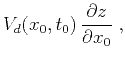
Conversion from time to depth coordinates and from $V_d(x_0,t_0)$ to $V(x,z)$ is a nontrivial inverse problem. The problem involves not only a coordinate transformation (Hatton et al., 1981; Larner et al., 1981) but also a correction for the geometrical spreading of image rays. As shown by Cameron et al. (2009), the problem can be reduced to solving an initial-value (Cauchy) problem for an elliptic PDE (partial differential equation), which is a classic example of a mathematically ill-posed problem. 
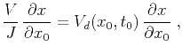
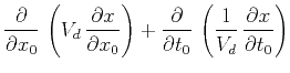
To arrive at this formulation, let us transform the system of equations 4-6 into the image-ray coordinate system. The system of equations for inverse functions takes the form (Li and Fomel, 2015)


$\displaystyle \left(\frac{\partial x}{\partial x_0}\right)^2 + \left(\frac{\partial z}{\partial x_0}\right)^2$ $\textstyle =$ $\displaystyle J^2\;,$ (11)
$\displaystyle \frac{\partial x}{\partial x_0}\,\frac{\partial x}{\partial t_0} + \frac{\partial z}{\partial x_0}\,\frac{\partial z}{\partial t_0}$ $\textstyle =$ $\displaystyle 0\;,$ (12)
$\displaystyle \left(\frac{\partial x}{\partial t_0}\right)^2 + \left(\frac{\partial z}{\partial t_0}\right)^2$ $\textstyle =$ $\displaystyle V^2\;,$ (13)

with boundary conditions $x(x_0,0) = x_0$ and $z(x_0,0) = 0$.

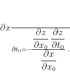
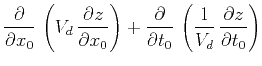
From equation 12, it follows that

\begin{displaymath}
\frac{\partial x}{\partial t_0} = -
\frac
{\displaysty...
...tial t_0}}
{\displaystyle \frac{\partial x}{\partial x_0}}\;.
\end{displaymath} (14)

Substituting this expression into equation 13 and using equation 11 leads to
$\displaystyle \frac{\partial x}{\partial t_0}$ $\textstyle =$ $\displaystyle V_d(x_0,t_0)\,\frac{\partial z}{\partial x_0}\;,$ (15)
$\displaystyle \frac{\partial z}{\partial t_0}$ $\textstyle =$ $\displaystyle \frac{V}{J}\,\frac{\partial x}{\partial x_0} =
V_d(x_0,t_0)\,\frac{\partial x}{\partial x_0}\;,$ (16)

where both $\partial z/\partial t_0$ and $\partial x/\partial x_0$ are assumed to remain positive (image rays propagate down and do not cross). Finally, decoupling the system by using the equivalence of the second-order mixed derivatives produces the following system of two linear elliptic PDEs:
$\displaystyle \frac{\partial}{\partial x_0}\,
\left(V_d\,\frac{\partial x}{\par...
...al}{\partial t_0}\,
\left(\frac{1}{V_d}\,\frac{\partial x}{\partial t_0}\right)$ $\textstyle =$ $\displaystyle 0\;,$ (17)
$\displaystyle \frac{\partial}{\partial x_0}\,
\left(V_d\,\frac{\partial z}{\par...
...al}{\partial t_0}\,
\left(\frac{1}{V_d}\,\frac{\partial z}{\partial t_0}\right)$ $\textstyle =$ $\displaystyle 0\;.$ (18)

Additional initial conditions,
$\displaystyle \left. \frac{\partial x}{\partial t_0}\right\vert _{t_0=0}$ $\textstyle =$ $\displaystyle 0\;,$ (19)
$\displaystyle \left. \frac{\partial z}{\partial t_0}\right\vert _{t_0=0}$ $\textstyle =$ $\displaystyle V_d(x_0,0)\;.$ (20)

specify that the image rays propagate down normal to the surface. If it were possible to solve system 17-18 directly using only initial conditions, the shape of image rays could be determined, and the true velocity could be estimated from equation 13. Unfortunately, this problem is mathematically ill-posed, which leads to numerical instability (Tikhonov and Arsenin, 1977). It can be approached, however, through regularization techniques (Cameron et al., 2009).

Li and Fomel (2015) develop robust time-to-depth conversion, which uses equations 4-6 in the Cartesian coordinate system and formulates time-to-depth conversion as a regularized least-squares optimization problem. Using linearization with respect to velocity perturbations Sripanich and Fomel (2018) reformulate equations 17-18 for fast time-to-depth conversion appropriate for handling weak lateral variations. Weak lateral variation assumption is important because in case of strong lateral variations, there is no longer a one-to-one mapping between image-ray coordinates and Cartesian coordinates, and the coordinate transformation will also have a zero determinant (at the caustics of the image-ray field). Using Sripanich and Fomel (2018), the squared Dix velocity converted to depth $w_d(x,z)$ is given as

\begin{displaymath}
w_d (x,z) \approx w_{dr}(x,z) + \left(\Delta x_0 (x,z) \time...
... (x,z) \times \frac{\partial w_d}{\partial t_0}(x,z) \right)~,
\end{displaymath} (21)

where $w_{dr}(x,z)$ denotes the $w_d(x_0,t_0)$ converted to depth based on the laterally homogeneous background assumption, and the derivatives with respect to $x_0$ and $t_0$ are evaluated first in the original $(x_0,t_0)$ coordinates followed by a similar conversion.


next up previous [pdf]

Next: Step 5. Velocity model Up: Workflow: Wave-equation time migration Previous: Step 3. Wave-equation time

2022-05-23