|
 |
 |
 | Wave-equation time migration |  |
![[pdf]](icons/pdf.png) |
Next: Workflow: Wave-equation time migration
Up: Fomel & Kaur: Wave-equation
Previous: Introduction
The phase information contained in seismic waves is governed by the
eikonal equation, which takes the form (Chapman, 2004)
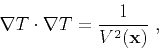 |
(1) |
where  is a point in space,
  is
traveltime from the source to , and
is
traveltime from the source to , and  is the
phase velocity. In an anisotropic medium, the phase velocity depends
additionally on the direction of traveltime gradient
is the
phase velocity. In an anisotropic medium, the phase velocity depends
additionally on the direction of traveltime gradient  . For simplicity, we limit the following discussion to the isotropic
case and two dimensions. Extensions to anisotropy and 3-D are possible
but would complicate the discussion. In 2-D,
. For simplicity, we limit the following discussion to the isotropic
case and two dimensions. Extensions to anisotropy and 3-D are possible
but would complicate the discussion. In 2-D,
 , and
the isotropic eikonal equation 1 can be written as
, and
the isotropic eikonal equation 1 can be written as
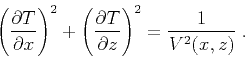 |
(2) |
The simplest wave equation that corresponds to eikonal
equation 1 is the acoustic wave equation
 |
(3) |
where  is a wavefield propagating with velocity
 . Equation 3 provides the basis for a variety of
wave-equation migration algorithms, from one-way wave extrapolation in
depth to two-way reverse-time migration (RTM) (Biondi, 2006; Etgen et al., 2009).
. Equation 3 provides the basis for a variety of
wave-equation migration algorithms, from one-way wave extrapolation in
depth to two-way reverse-time migration (RTM) (Biondi, 2006; Etgen et al., 2009).
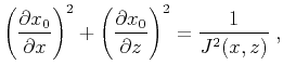
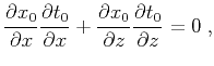
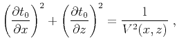
Consider a family of image rays (Hubral, 1977), traced
orthogonal to the surface. Image-ray coordinates  and
and  as
functions of the Cartesian coordinates
as
functions of the Cartesian coordinates  and
and  satisfy the
following system of partial differential equations (Cameron et al., 2007):
satisfy the
following system of partial differential equations (Cameron et al., 2007):
with boundary conditions  and
and
 . Equation 6 is the familiar eikonal
equation 2. Equation 5 expresses the
orthogonality of rays and wavefronts in an isotropic
medium. Equation 4 defines the quantity
. Equation 6 is the familiar eikonal
equation 2. Equation 5 expresses the
orthogonality of rays and wavefronts in an isotropic
medium. Equation 4 defines the quantity  as the
geometrical spreading of image rays.
as the
geometrical spreading of image rays.
Applying a change of variables from  to
to  transforms eikonal equation 2 to the
coordinate system of image rays and leads to an
elliptically anisotropic eikonal equation which is
transforms eikonal equation 2 to the
coordinate system of image rays and leads to an
elliptically anisotropic eikonal equation which is
 |
(7) |
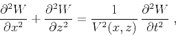
The corresponding wave equation is given by
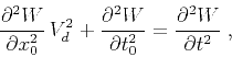 |
(8) |
where  . Equation 8 is a particular version of
the more general Riemannian coordinate transformation analyzed
by Sava and Fomel (2005). Some other versions of Riemannian coordinate transformations are analysed by Shragge (2008); Shragge and Shan (2008). Note that at the surface of observation
. Equation 8 is a particular version of
the more general Riemannian coordinate transformation analyzed
by Sava and Fomel (2005). Some other versions of Riemannian coordinate transformations are analysed by Shragge (2008); Shragge and Shan (2008). Note that at the surface of observation
 , the solution of equation 8 coincides
geometrically with the solution of the original Cartesian
equation 3.
, the solution of equation 8 coincides
geometrically with the solution of the original Cartesian
equation 3.
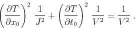
The significance of equation 8 lies in the following
fact established by Cameron et al. (2007). When time migration is performed using
coordinates and and the conventional traveltime approximation based
on the Taylor expansion of diffraction traveltime around the image
ray, such as the classic hyperbolic approximation
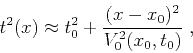 |
(9) |
the coefficient  appearing in equation 8 is simply
related to time-migration velocity
appearing in equation 8 is simply
related to time-migration velocity  appearing in
equation 9. More specifically,
appearing in
equation 9. More specifically,
![\begin{displaymath}
V_d^2(x_0,t_0) = \frac{V^2}{J^2} = \frac{\partial \left[t_0\,V_0^2(x_0,t_0)\right]}{\partial t_0}\;.
\end{displaymath}](img36.png) |
(10) |
Following Cameron et al. (2008a), we call Dix velocity because it
corresponds to the classic Dix inversion applied to the time-migration
velocity (Dix, 1955). In the absence of lateral
velocity variations (a  medium), image rays do not spread;
therefore,
medium), image rays do not spread;
therefore,  ,
,  and corresponds to true velocity in the
medium, and corresponds to root-mean-square (RMS) velocity. In
the presence of lateral velocity variations, the conversion between
time-migration coordinates and true Cartesian coordinates is more
complicated (Cameron et al., 2008a; Li and Fomel, 2015; Bevc et al., 1995). However, to
extrapolate seismic wavefields in image-ray coordinates using
equation 8, it is sufficient to use an estimate of the Dix
velocity , which is readily available from conventional
time-domain processing and equation 10.
and corresponds to true velocity in the
medium, and corresponds to root-mean-square (RMS) velocity. In
the presence of lateral velocity variations, the conversion between
time-migration coordinates and true Cartesian coordinates is more
complicated (Cameron et al., 2008a; Li and Fomel, 2015; Bevc et al., 1995). However, to
extrapolate seismic wavefields in image-ray coordinates using
equation 8, it is sufficient to use an estimate of the Dix
velocity , which is readily available from conventional
time-domain processing and equation 10.
|
|
|
|
| Wave-equation time migration | |
|
Next: Workflow: Wave-equation time migration
Up: Fomel & Kaur: Wave-equation
Previous: Introduction
2022-05-23