 |
 |
 |
 | A robust approach to time-to-depth conversion and interval velocity
estimation from time migration in the presence of lateral velocity variations |  |
![[pdf]](icons/pdf.png) |
Next: Appendix D: Analytical expressions
Up: Li & Fomel: Time-to-depth
Previous: Appendix B: The Fréchet
In order to derive the time-to-depth conversion analytically, we first trace image rays in the depth
coordinate for  and
and  . Then we carry out a direct inversion to find
  and
and
 . The Dix velocity can be obtained at last following equations 3 and 4.
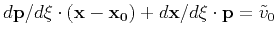
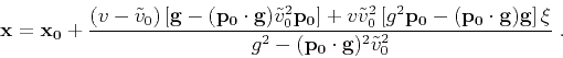
Continuing from equation 15, we write the velocity in a coordinate relative to the image ray
 |
(39) |
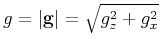
where
![$\mathbf{g} = [g_z,g_x]^T$](img164.png) and
and
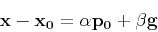
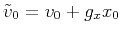 . At the starting point, image ray satisfies
![\begin{displaymath}
\left\{ \begin{array}{lcl}
\mathbf{x_0} & = & [0, x_0]^T\;, ...
...ilde{v}_0^{-1}, 0]^T\;, \\
t_0 & = & t\;.
\end{array} \right.
\end{displaymath}](img166.png) |
(40) |
Here we denote ray parameter
 and
and  is the ray parameter at source. The
Hamiltonian for ray tracing reads
is the ray parameter at source. The
Hamiltonian for ray tracing reads
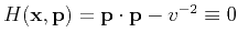 .
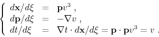
The corresponding ray tracing system is (Cervený, 2001):
.
The corresponding ray tracing system is (Cervený, 2001):
 |
(41) |
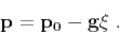
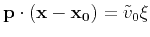
Equation C-1 indicates
 , which means
 can be
integrated analytically and provides
can be
integrated analytically and provides
 |
(42) |
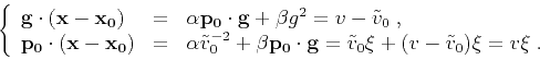
From the eikonal equation and considering
 and
and
 , we have
 |
(43) |
Integrating equation C-5 over  gives
gives
 |
(44) |
Meanwhile, combining equations C-1 and C-3, we find
 ,
i.e.,
,
i.e.,
 . Suppose
 |
(45) |
then
 |
(46) |
Solving equation C-8 provides
 and
and  , which after substituting into
equation C-7 leads to
, which after substituting into
equation C-7 leads to
 |
(47) |
Note equation C-2 states
 and thus equations
C-4, C-6 and C-9 can be further simplified.
and thus equations
C-4, C-6 and C-9 can be further simplified.
To connect depth- and time-domain attributes, we first invert equation C-6 such that is
expressed by  and
and 
 |
(48) |
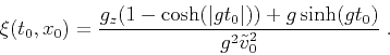
Next, we insert equations C-5 and C-10 into C-9 in order to change its
parameterization from  to
to  . The result is written for the
  and
and  components of
 separately, as follows:
 |
(49) |
![\begin{displaymath}
z (t_0,x_0) = \frac{\tilde{v}_0 \left[ g_z (1 - \cosh (g t_0...
... (g t_0) \right]}
{g (g \cosh (g t_0) - g_z \sinh (g t_0))}\;.
\end{displaymath}](img191.png) |
(50) |
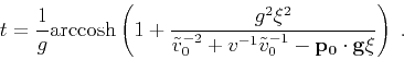
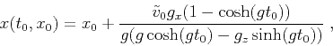
Inverting equations C-11 and C-12 results in
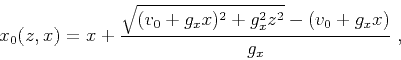 |
(51) |
![\begin{displaymath}
t_0 (z,x) = \frac{1}{g} \mathrm{arccosh} \left\{ \frac{g^2 \...
...2 + g_x^2 z^2}
+ g_z z \right] - v g_z^2}{v g_x^2} \right\}\;.
\end{displaymath}](img192.png) |
(52) |
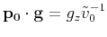
In the last step, we derive the analytical formula for the Dix velocity. Note that from equation
C-13
 , i.e., there is no geometrical spreading. The image rays are circles parallel
to each other. Therefore according to equation 3
, i.e., there is no geometrical spreading. The image rays are circles parallel
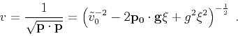
to each other. Therefore according to equation 3  and is found by combining equations
C-5 and C-10
and is found by combining equations
C-5 and C-10
 |
(53) |
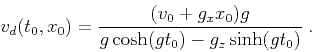
The time-migration velocity  , on the other hand, is
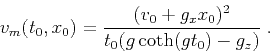 |
(54) |
|
|
|
|
| A robust approach to time-to-depth conversion and interval velocity
estimation from time migration in the presence of lateral velocity variations | |
|
Next: Appendix D: Analytical expressions
Up: Li & Fomel: Time-to-depth
Previous: Appendix B: The Fréchet
2015-03-25