Fast time-to-depth conversion and interval velocity estimation in the case of weak lateral variations

Linear sloth model

We first test the proposed method using a synthetic model with known analytical time-to-depth conversion solutions. In this model, the exact velocity squared is given by

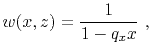$$w(x,z) = \frac{1}{1-q_x x}~,$$ (22)

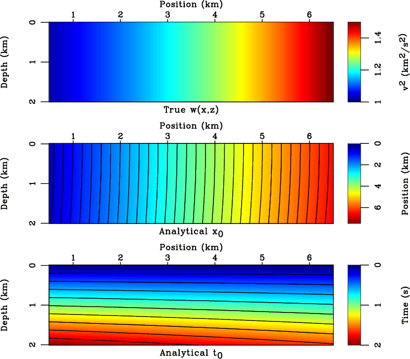
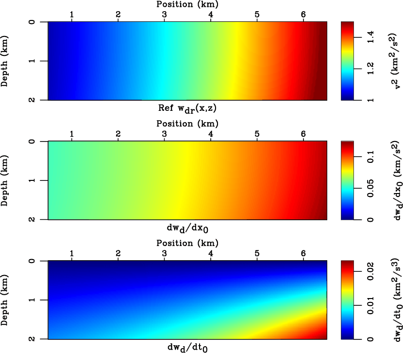
where $q_x=0.052$ , which gives a maximum of 25$\%$ changes in lateral velocity along the 7 $km$ lateral extent of the model. The analytical solutions to time-to-depth conversion in this particular type of model were presented by Li and Fomel (2015). Figure 3 shows the true interval velocity of the model (equation 22), and the analytical $x_0$ and $t_0$ overlaid by the contours indicating image rays and propagating image wavefront. Other inputs for the proposed conversion method are shown in Figure 4. 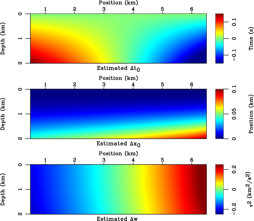We choose the reference $w_r(z)$ background to be the central trace of the reference $w_{dr}(x,z)$ , which is constant in this case. The estimated results are shown in Figure 5 and their corresponding errors in comparison with the analytical values are shown in Figure 6. The errors appear to be generally small indicating a good accuracy for all estimated parameters but increase closer to the edges of the model, which are further away from the chosen reference $w_r(z)$ .

model-slow
Figure 3. The true velocity squared (top) of the linear sloth model (equation 22). Analytical $x_0$ (middle) is overlaid by image rays. Analytical $t_0$ (bottom) is overlaid by contours showing propagating image wavefront.

input-slow
Figure 4. Inputs of the proposed time-to-depth conversion for the linear gradient model. The last input $w_r(z)$ (not shown here) is taken to be the central trace of $w_{dr}(x,z)$ (top) in this case.

estcompare-slow
Figure 5. The estimated values of $\Delta x_0$ , $\Delta t_0$ , $\Delta w$ in the linear sloth model (equation 22).

errcompare-slow
Figure 6. The errors of the estimated values of $\Delta x_0$ , $\Delta t_0$ , $\Delta w$ in comparison with the true values in the linear sloth model (equation 22). The errors are small for all estimated parameters indicating a good accuracy of the proposed method.

Fast time-to-depth conversion and interval velocity estimation in the case of weak lateral variations