Dip steering and local SVD

Supposing the events in a processing window have one slope, dip steering algorithm aims to flatten the dipping events by shifting each trace such that the flattened events are suitable for applying a GSVD based denoising approach, as shown in equation 4. This flattening strategy is called dip steering (Bekara and van der Baan, 2007). After removing noise, applying an inverse flattening to the data in the processing window can obtain the denoised data. We refer to those denoising approaches that apply a GSVD in the dip-steering flattened domain as local SVD (LSVD). The time shifts for each trace in order to flatten the events are obtained by selecting the time delays that can maximize cross-correlation between each trace and a reference trace.

$$\tau_n = \arg\max_{\tau} \sum_{m=\min(1-\tau,1)}^{\max(M_w,M_w-\tau)} r(m)d(m+\tau,n),$$ (5)

where $\tau_n$ is the optimal time shift for $n$th trace in the processing window, $M_w$ denotes the number of time samples in the processing window and $r(m)$ denotes the $m$th sample of the reference trace and $d(m,n)$ denotes the data value in $m$th sample and $n$th trace. $\tau_n>0$ corresponds to shifting trace downward with respect to the reference trace, and $\tau_n<0$ corresponds to shifting trace upward.

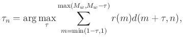
As can be seen from the equation 5, the selection of reference trace is crucial for the effectiveness of LSVD. It can be chosen as random trace in the processing window if the noise level is not high, or can be chosen as a stacked trace after normal-moveout (NMO) of common-midpoint gathers. Bekara and van der Baan (2007) proposed an iterative strategy for selecting the optimal reference trace stating that the resulting shifted traces are stacked after each cross-correlation pass for updating the new reference traces and the process of cross-correlation, shifting, and stacking is repeated until the process converges. Figure 1 shows a demonstration for dip steering and the processes of LSVD. Figure 1a is the original noisy dipping event. Figure 1b denotes the flattened event after forward dip steering. Figure 1c shows the LSVD denoised result by choosing only one singular value. The final denoised result after inverse dip steering on Figure 1c is shown in Figure 1d. The time shifts after the optimizing equation 5 are shown in Figure 2. The reference trace is simply chosen as the first trace of the original data, as shown in Figure 1a.

dn,dh,dhc,dc
Figure 1. Demonstration for dip steering and LSVD. (a) Noisy dip reflector. (b) Flattened event using dip steering. (c) SVD denoised result by selecting only one eigen-image. (d) Denoised data after inverse dip steering.

shift
Figure 2. Time shifts for each trace for the forward dip steering as shown in Figure 1 (reference trace selected as the left trace in Figure 1a).