|
|
|
|
Lowrank seismic wave extrapolation on a staggered grid |
Next we use the method of manufactured solutions (MMS) (Salari and Knupp, 2000) to analyze numerical error of the proposed methods. MMS provides an approach to designing exact reference solutions for wave equations in heterogeneous media. We couple the use of manufactured solutions with mesh refinement to plot the error curve for each method. To begin our investigation, we consider the system of 1D first order wave equations,
For numerical solution, accuracy is often affected by various factors. In this study, we examine the numerical error of the proposed methods when using different temporal and spatial discretization and wavelets of different dominant frequencies. The velocity we used here increases with ![]() , defined as
, defined as
![]() . Its gradient is
. Its gradient is
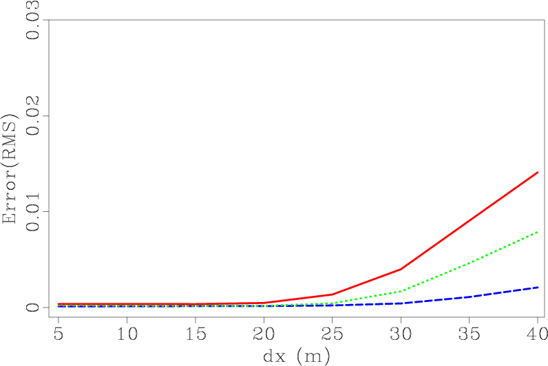
![]() correspondingly. We use constant density in this experiment. Figure 6a shows the RMS errors of the wavefields for different time interval. For all these calculations, we keep space interval
correspondingly. We use constant density in this experiment. Figure 6a shows the RMS errors of the wavefields for different time interval. For all these calculations, we keep space interval
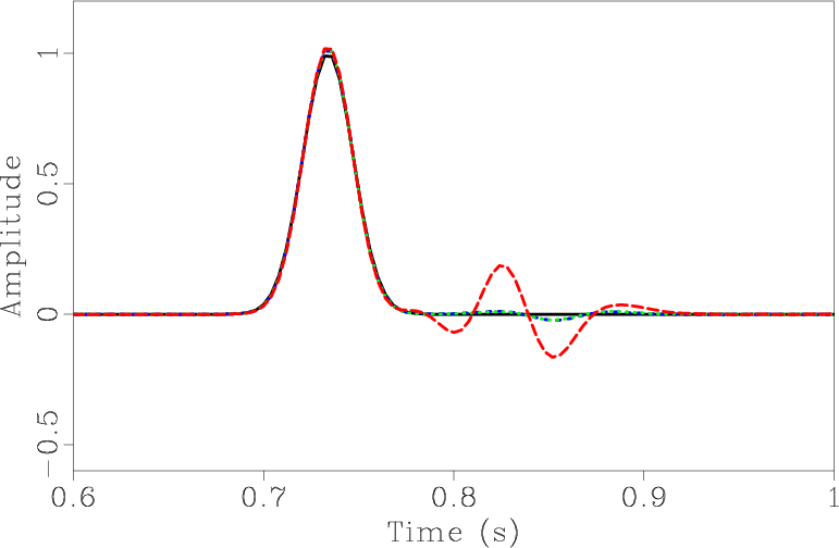
![]() as constant. The blue dashed line and green dotted line indicate the errors of SGL method and SGLFD method respectively, while red solid line plots the errors of the traditional SGFD method. Compared with the traditional SGFD method, the proposed lowrank methods correct the distortion caused by increasing
as constant. The blue dashed line and green dotted line indicate the errors of SGL method and SGLFD method respectively, while red solid line plots the errors of the traditional SGFD method. Compared with the traditional SGFD method, the proposed lowrank methods correct the distortion caused by increasing ![]() . They exhibit a high accuracy in time. Figure 6b shows the recorded trace at the
. They exhibit a high accuracy in time. Figure 6b shows the recorded trace at the ![]() of
of ![]() for
for
![]() .The black solid line corresponds to the exact solution generated by MMS. The colors of remaining lines has the same meaning as in Figure 6a. Numerical dispersion is more visible when
.The black solid line corresponds to the exact solution generated by MMS. The colors of remaining lines has the same meaning as in Figure 6a. Numerical dispersion is more visible when ![]() is increased; this effect is much less significant in our methods.
is increased; this effect is much less significant in our methods.

|
|---|
|
et,trec19
Figure 6. (a) RMS errors as function of time interval. (b) Recorded data for |
|
|
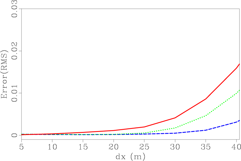
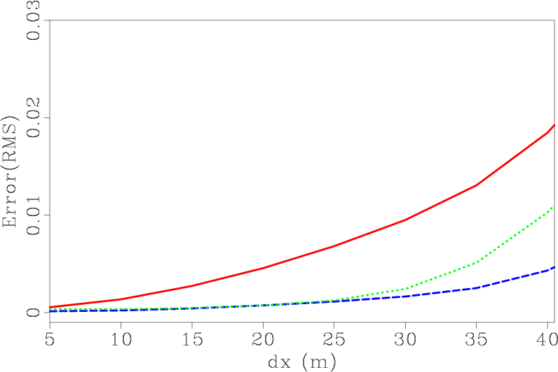
Figure 7a shows the RMS errors of the wavefields for
different space intervals. We use a small time interval
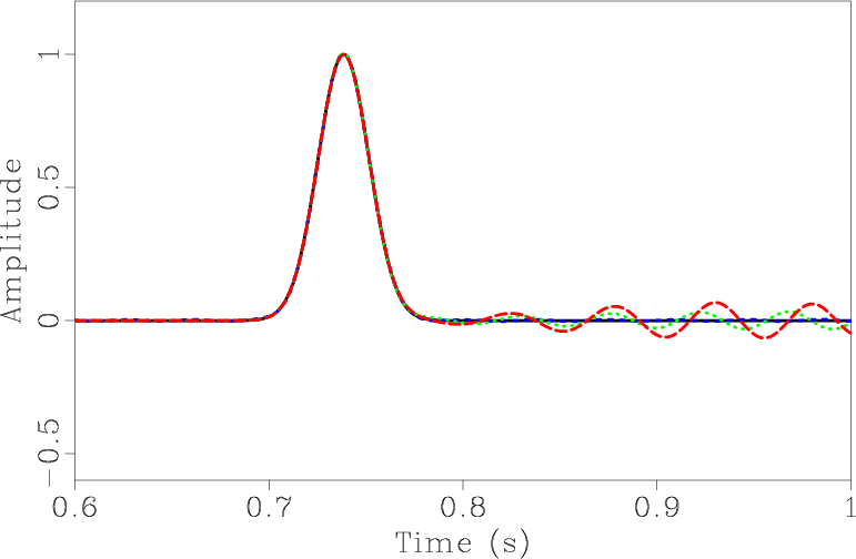
![]() to keep time error small. Figure 7b shows the recorded data for
to keep time error small. Figure 7b shows the recorded data for
![]() . The first-order
. The first-order ![]() -space operators
(equation 9) have a high accuracy in space which
make the error of SGL method increase slowly when
-space operators
(equation 9) have a high accuracy in space which
make the error of SGL method increase slowly when ![]() increase. The coefficients of the SGLFD are obtained by applying least-squares fitting to the SGL method. The error from the least-squares fitting make SGLFD method less accurate than SGL method. On the other hand, the
coefficients of lowrank FD are optimized and auto-adapted to variations in velocity, which makes it significantly more accurate than SGFD method.
increase. The coefficients of the SGLFD are obtained by applying least-squares fitting to the SGL method. The error from the least-squares fitting make SGLFD method less accurate than SGL method. On the other hand, the
coefficients of lowrank FD are optimized and auto-adapted to variations in velocity, which makes it significantly more accurate than SGFD method.
|
|---|
|
em,mrec7
Figure 7. (a) RMS errors as function of space interval. (b) Recorded data for |
|
|
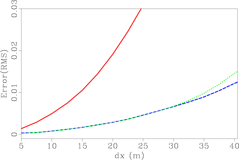
In applications of seismic wave extrapolation, temporal and spatial intervals are often increased at a
certain ratio for saving computational cost. Figure 8
show the error curves for a temporal and spatial refinement study where
both ![]() and
and ![]() are increased
simultaneously. We define the Courant-Friedrichs-Lewy (CFL) number as
are increased
simultaneously. We define the Courant-Friedrichs-Lewy (CFL) number as
![]() to specify the stability condition, where
to specify the stability condition, where ![]() is the maximum velocity. Figure 8a shows the RMS errors for
is the maximum velocity. Figure 8a shows the RMS errors for
![]() . Figure 8b shows the RMS error of
. Figure 8b shows the RMS error of
![]() , while figure 8c for
, while figure 8c for
![]() . The color of the lines has the same meaning as indicated before. We can see that the errors increase with the CFL number
. The color of the lines has the same meaning as indicated before. We can see that the errors increase with the CFL number ![]() . This increase is especially significant for SGFD method. Both SGL and SGLFD methods keep high accuracy for a larger scale of temporal and spatial intervals than SGFD.
. This increase is especially significant for SGFD method. Both SGL and SGLFD methods keep high accuracy for a larger scale of temporal and spatial intervals than SGFD.
|
|---|
|
ea2,ea4,ea8
Figure 8. RMS errors for CFL number (a) |
|
|
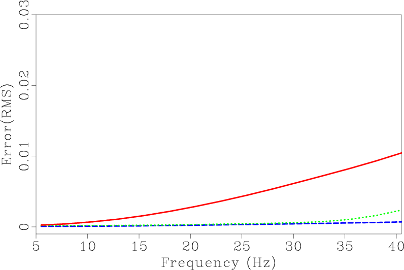
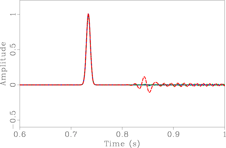
Seismic exploration techniques, such as prestack depth migration or FWI, need the modeling engine which remains highly accurate for a wide band seismic wavelet. The numerical dispersion can be serious for a high frequency source. Figure 9a compares the accuracy of different methods for different source frequencies. The meanings of different line colors are the same as before. Figure 9b shows the recorded data with source frequency of ![]() . It can be seen that the SGFD method has a visible dispersion, while SGL and SGLFD methods remain almost dispersion free.
. It can be seen that the SGFD method has a visible dispersion, while SGL and SGLFD methods remain almost dispersion free.
|
|---|
|
fre,frec15
Figure 9. (a) RMS errors as function of dominant frequency of source wavelet. (b) Recorded data for frequency of |
|
|
|
|
|
|
Lowrank seismic wave extrapolation on a staggered grid |
![\begin{displaymath}\begin{array}{l} \displaystyle s_u(x,t) = 2\lambda^2[x-x_0-v(...
...2[x-x_0-v(x)t][v(x)+\rho(x)v^2(x)(v'(x)t-1)]p(x,t). \end{array}\end{displaymath}](img131.png)