|
|
|
|
Lowrank seismic wave extrapolation on a staggered grid |
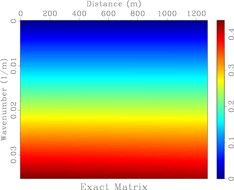
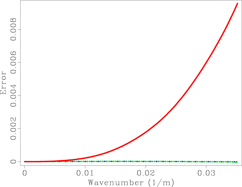
We first use a simple 1-D example shown in Figure 4 to demonstrate the accuracy of the SGL method and SGLFD method when they are used to calculate the partial derivatives in equation 9. The velocity increases linearly from 1000 to 2275 m/s. The rank is 2 for lowrank decomposition, assuming 1 ms time step. The exact ![]() -space operator
-space operator
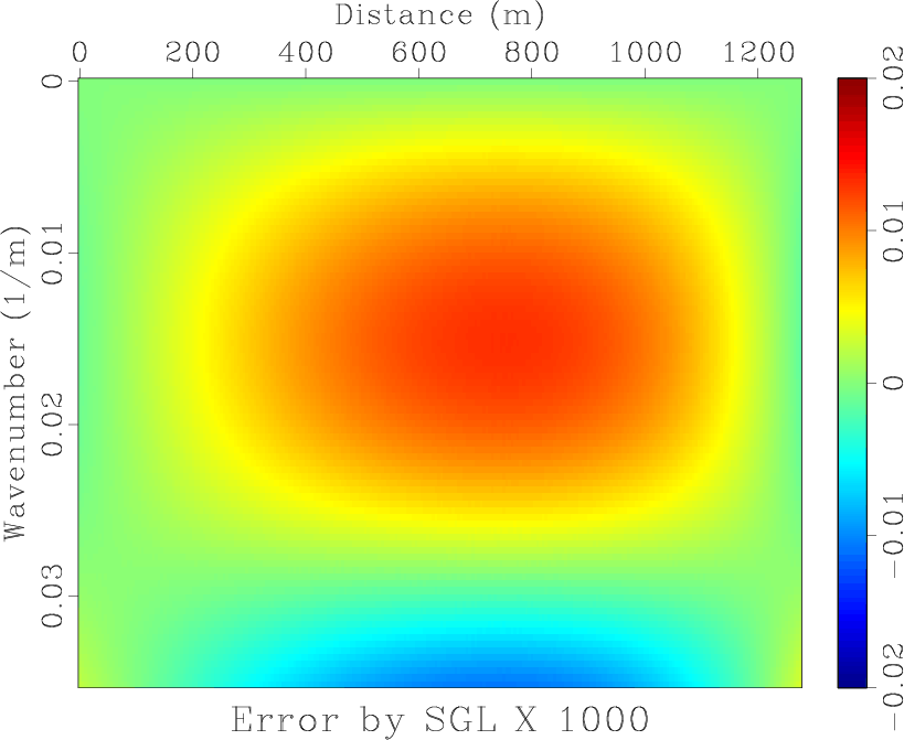
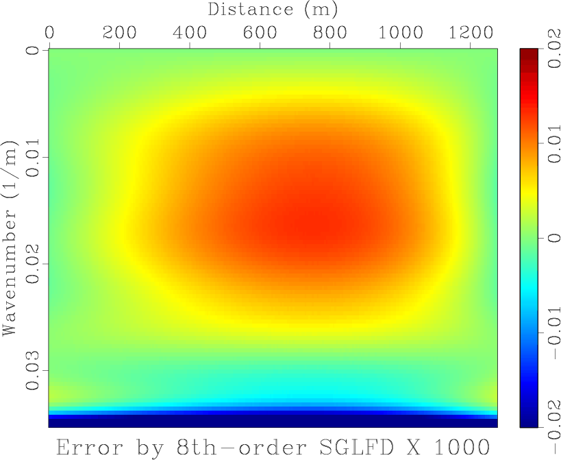
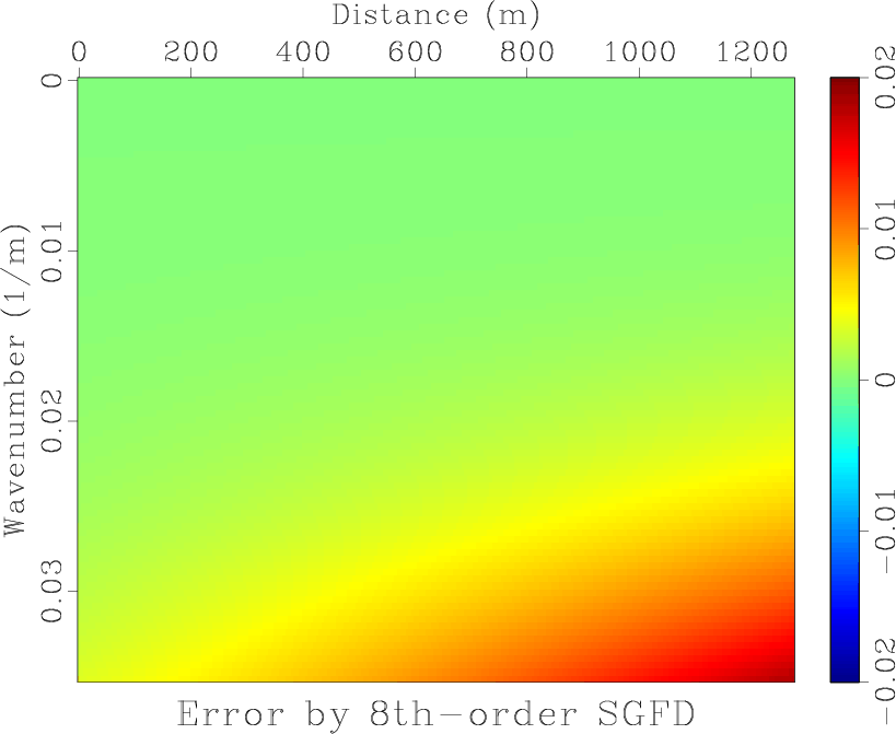
![]() in equation 9 is shown in Figure 4a. Figures 4b, 4c and 4d display errors of approximation operators of SGL, SGLFD and conventional staggered grid finite-difference (SGFD), respectively. Figure 5 shows the middle column of the error matrix. The errors of SGL and SGLFD are significantly smaller than that of SGFD.
in equation 9 is shown in Figure 4a. Figures 4b, 4c and 4d display errors of approximation operators of SGL, SGLFD and conventional staggered grid finite-difference (SGFD), respectively. Figure 5 shows the middle column of the error matrix. The errors of SGL and SGLFD are significantly smaller than that of SGFD.
|
|---|
|
Mexact,Mlrerr,Mapperr,Mfd10err
Figure 4. (a) |
|
|
|
|---|
|
slicel
Figure 5. Middle column of the error matrix. Blue dashed line: SGL operator. Green dotted line: the 8th order SGLFD operator. Red solid line: the 8th order SGFD operator. |
|
|
|
|
|
|
Lowrank seismic wave extrapolation on a staggered grid |