|
|
|
|
Lowrank seismic wave extrapolation on a staggered grid |
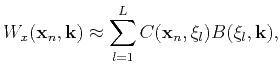
Approximation 12 can also be used to design accurate finite-difference schemes. Here we extend the lowrank finite-difference method (Song et al., 2013) to first-order ![]() -space operators. Note that
-space operators. Note that
![]() in equation 13 is a matrix related only to wavenumber
in equation 13 is a matrix related only to wavenumber
![]() . It can be further decomposed as follows:
. It can be further decomposed as follows:
Equation 17 corresponds to the procedure of finite-difference scheme for calculating the ![]() -space operator. The vector
-space operator. The vector
![]() provides stencil information, and
provides stencil information, and
![]() stores the corresponding coefficients. A similar derivation can be applied to the remaining partial derivative operators in equation 9. We call this staggered grid lowrank finite-differences (SGLFD) method.
stores the corresponding coefficients. A similar derivation can be applied to the remaining partial derivative operators in equation 9. We call this staggered grid lowrank finite-differences (SGLFD) method.
While the SGL method (equation 13) is proposed by applying lowrank approximation to the ![]() space method on a staggered grid (equation 9), SGLFD (equation 17) is a further approximation of SGL. Theoretically, the SGLFD method using a longer stencil reaches higher accuracy. It is hard to derive stability condition for SGL. However, applying Von Neumann stability analysis, we can easily obtain a sufficient condition of stability for SGLFD as
space method on a staggered grid (equation 9), SGLFD (equation 17) is a further approximation of SGL. Theoretically, the SGLFD method using a longer stencil reaches higher accuracy. It is hard to derive stability condition for SGL. However, applying Von Neumann stability analysis, we can easily obtain a sufficient condition of stability for SGLFD as
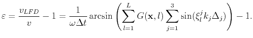
Next, we use the plane wave theory to evaluate numerical dispersion for SGLFD method. Inserting the plane wave solution,
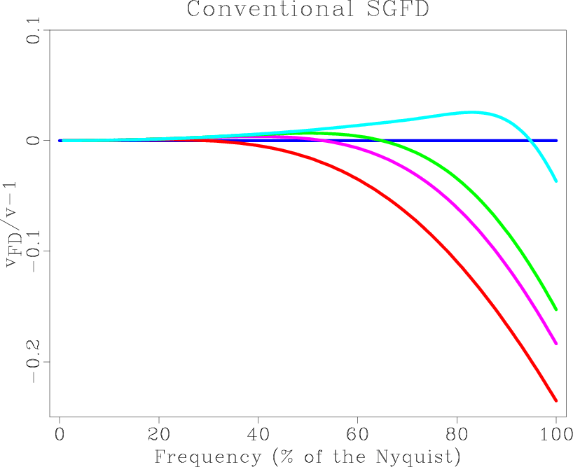
Figure 1 shows the variation of
![]() with frequency for different order. This figure demonstrates that dispersion decrease with the increase of the order for both SGFD and SGLFD method. Note that for SGFD method increase of order decreases the magnitude of the dispersion error without increasing the area where
with frequency for different order. This figure demonstrates that dispersion decrease with the increase of the order for both SGFD and SGLFD method. Note that for SGFD method increase of order decreases the magnitude of the dispersion error without increasing the area where
![]() nearly equals 0. Compared with the SGFD method, the SGLFD method is high accurate in a wider range of wavenumber.
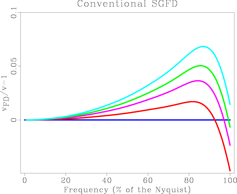
Figure 2 shows the variation of the
nearly equals 0. Compared with the SGFD method, the SGLFD method is high accurate in a wider range of wavenumber.
Figure 2 shows the variation of the
![]() with frequency for difference time interval. From this figure, we can see that the dispersion becomes stronger when the SGFD method uses larger time interval. Moreover, if a large time interval is used, like
with frequency for difference time interval. From this figure, we can see that the dispersion becomes stronger when the SGFD method uses larger time interval. Moreover, if a large time interval is used, like
![]() in this example, the SGFD method will be unstable. However, for the SGLFD method, its dispersion mainly depends on the frequency. Compared with the SGFD method, the SGLFD method keeps high accuracy for different time intervals (up to
in this example, the SGFD method will be unstable. However, for the SGLFD method, its dispersion mainly depends on the frequency. Compared with the SGFD method, the SGLFD method keeps high accuracy for different time intervals (up to ![]() of the Nyquist frequency).
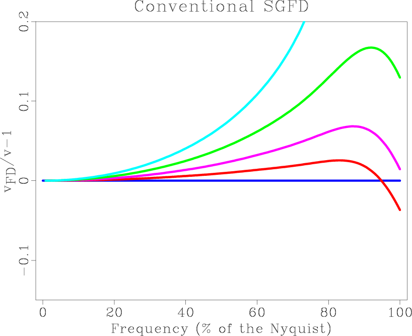
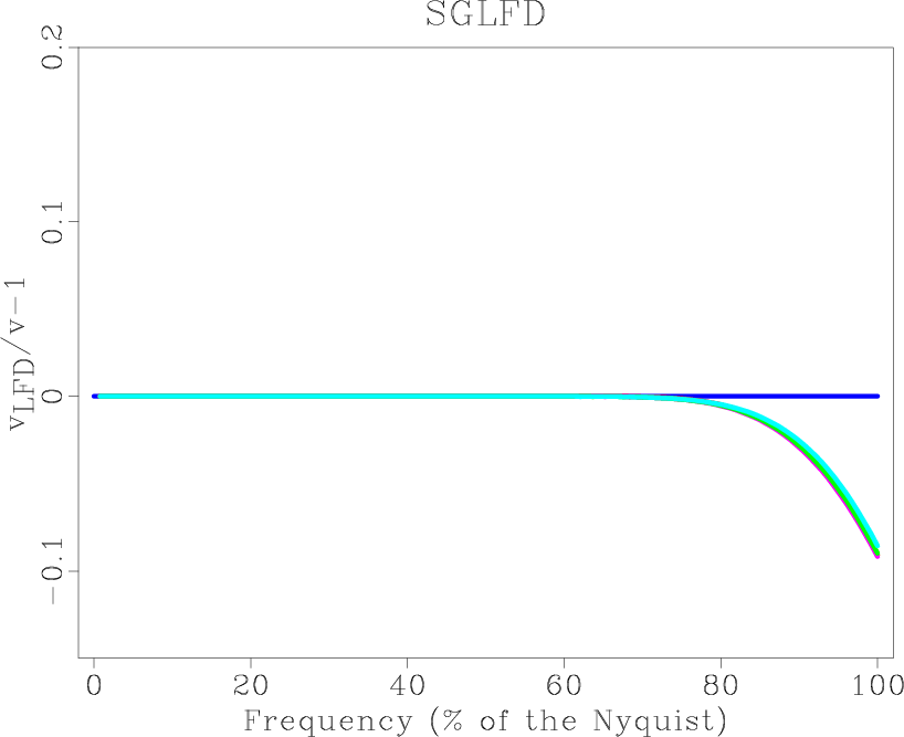
Figure 3 illustrates the effect of velocity on dispersion. Note that for the SGFD method, its dispersion curves change greatly with the variation of velocity. Compared with the SGFD method, the SGLFD method is more stable and accurate in a wider range of frequency(up to
of the Nyquist frequency).
Figure 3 illustrates the effect of velocity on dispersion. Note that for the SGFD method, its dispersion curves change greatly with the variation of velocity. Compared with the SGFD method, the SGLFD method is more stable and accurate in a wider range of frequency(up to ![]() of the Nyquist frequency).
In the previous examples, we used least squares to fit to nearly the
of the Nyquist frequency).
In the previous examples, we used least squares to fit to nearly the ![]() of the Nyquist frequency.
of the Nyquist frequency.

|
|---|
|
Mfd,Mlr
Figure 1. Plot of |
|
|
|
|---|
|
Mfdt,Mlrt
Figure 2. Plot of |
|
|

|
|---|
|
Mfdv,Mlrv
Figure 3. Plot of |
|
|
|
|
|
|
Lowrank seismic wave extrapolation on a staggered grid |
![\begin{displaymath}\begin{array}{l} \displaystyle \frac{\partial p(\mathbf{x},t)...
...\Delta_j})\mathbf{F}\left[p(\mathbf{x},t)\right]] . \end{array}\end{displaymath}](img102.png)
![$\displaystyle \displaystyle \frac{\partial p(\mathbf{x},t)}{\partial^+x} \appro...
...c{1}{2}\sum\limits_{l=1}^LG(\mathbf{x},l)[P(\mathbf{x}_R,t)-P(\mathbf{x}_L,t)],$](img109.png)