Lowrank seismic wave extrapolation on a staggered grid

Lowrank approximation for first-order extrapolation operators

In this section, we apply lowrank decomposition to approximate the extrapolation operator in equation 9. As indicated by Fomel et al. (2013b,2010), the mixed-domain matrix in equation 9, taking $$\frac{\partial p(\mathbf{x},t)}{\partial^+x}$$ as an example,

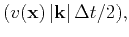$$W_x(\mathbf{x}, \mathbf{k}) = k_x (v(\mathbf{x})\left\vert\mathbf{k}\right\vert\Delta t/2),$$ (11)

can be efficiently decomposed into a separated representation as follows:

$$W_x(\mathbf{x}, \mathbf{k}) \approx \sum\limits_{m=1}^M\sum\limits_{n=1}^N W_x(\mathbf{x}, \mathbf{k}_m)a_{mn}W_x(\mathbf{x}_n, \mathbf{k}),$$ (12)

where $W_x(\mathbf{x}, \mathbf{k}_m)$ is a submatrix of $W_x(\mathbf{x}, \mathbf{k})$ which consists of selected columns associated with $\mathbf{k}_m$ ; $W_x(\mathbf{x}_n, \mathbf{k})$ is another submatrix that contains selected rows associated with $\mathbf{x}_n$ ; and $a_{nm}$ stands for middle matrix coefficients. The numerical construction of the separated representation in equation 12 follows the method of Engquist and Ying (2009).

Using representation 12, we can calculate $$\frac{\partial p(\mathbf{x},t)}{\partial^+x}$$ using a small number of fast Fourier transforms (FFTs), because

$$\displaystyle \frac{\partial p(\mathbf{x},t)}{\partial^+x} \appro... ...x/2}W_x(\mathbf{x}_n, \mathbf{k})\mathbf{F}\left[p(\mathbf{x},t)\right]\right].$$ (13)

The same lowrank decomposition approach can be applied to the remaining three partial derivative operators in equation 9. Evaluation of equation 13 only needs $N$ inverse FFTs, whose computational cost is 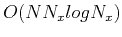$O(NN_xlogN_x)$ . However a straightforward application of equation 9 needs computational cost of $O(N^2_x)$ , where $N_x$ is the total size of the space grid. $N$ is related to the rank of the decomposed mixed-domain matrix 12, which is usually significantly smaller than $N_x$ . Note that the number of FFTs $N$ also depends on the given error level of lowrank decomposition with a predetermined $\Delta t$ . Thus a complex model or increasing the time interval size $\Delta t$ may increase the rank of the approximation matrix and correspondingly $N$ . In the numerical examples in this paper, the values of rank are usually between $2$ and $4$ . Lowrank decomposition saves cost in calculating equations 9 and 10. We propose to apply it for seismic wave extrapolation in variable velocity and density media on a staggered grid. We call this method staggered grid lowrank(SGL) method.

Lowrank seismic wave extrapolation on a staggered grid