|
|
|
|
Relative time seislet transform |
Next: RT formulation of prediction Up: Theory Previous: Reviews of the 2D
|
|
|
|
Relative time seislet transform |
Using linear operator notation, PWD operation is defined as
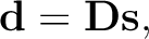 |
(5) |
![$\mathbf{s} =[\mathbf{s}_1 \,\mathbf{s}_2 \,\cdots\, \mathbf{s}_N]^T$](img17.png) is a collection of seismic traces and
is a collection of seismic traces and
 denotes the residual from
destruction.
denotes the residual from
destruction.
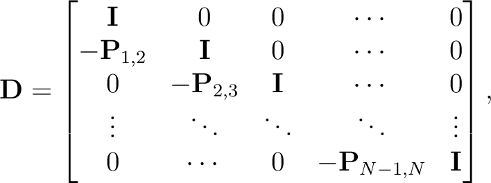
 is the destruction operator defined as
where
is the destruction operator defined as
where
 denotes the identity matrix and
 is
an operator that predicts the
is
an operator that predicts the  -th trace from the
  -th trace
according to the local slope of seismic event or seismic horizon.
-th trace
according to the local slope of seismic event or seismic horizon.
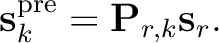
By a simple recursion, a trace can be predicted utilizing a distant trace.
For example,
 , predicting the
  -th trace from the
  -th
trace, is defined as
-th
trace, is defined as
 , given a reference trace
is accomplished by
After determining the prediction operators in equation 6 by PWD,
the predictive painting algorithm recursively spreads information from a
reference trace to the whole seismic data volume by following local slopes
using equation 8.
If the information spread by the predictive painting are the time
coordinates, an RT volume is easily computed.
, given a reference trace
is accomplished by
After determining the prediction operators in equation 6 by PWD,
the predictive painting algorithm recursively spreads information from a
reference trace to the whole seismic data volume by following local slopes
using equation 8.
If the information spread by the predictive painting are the time
coordinates, an RT volume is easily computed.
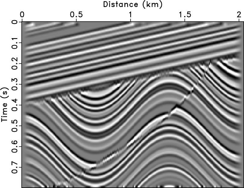
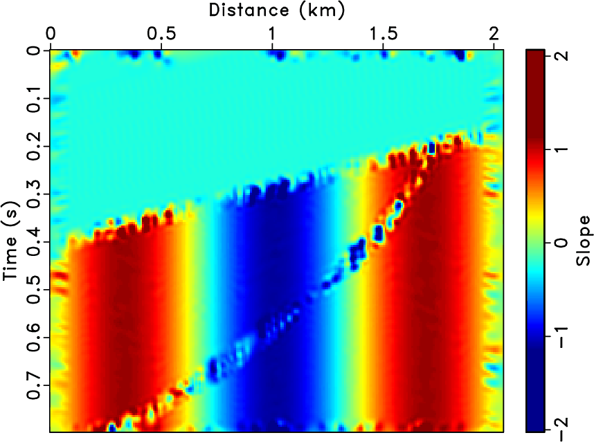
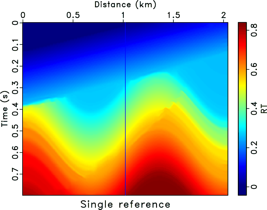
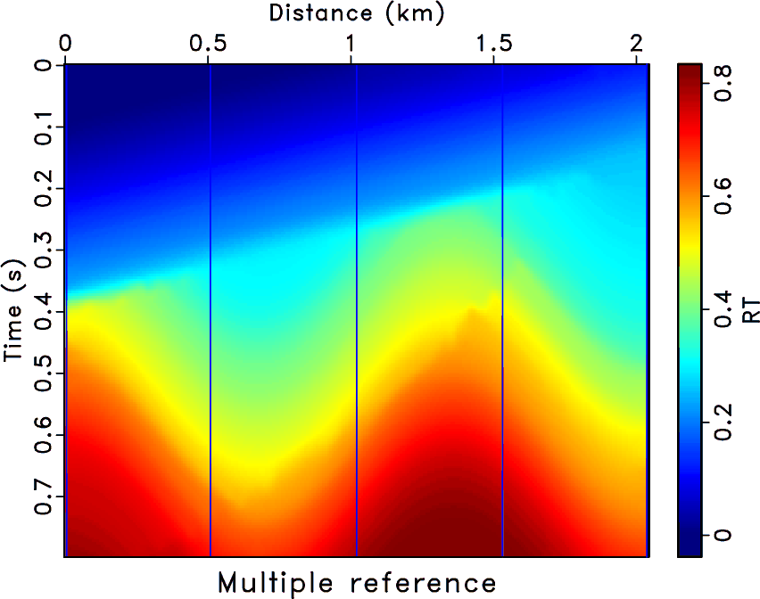
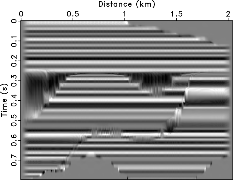
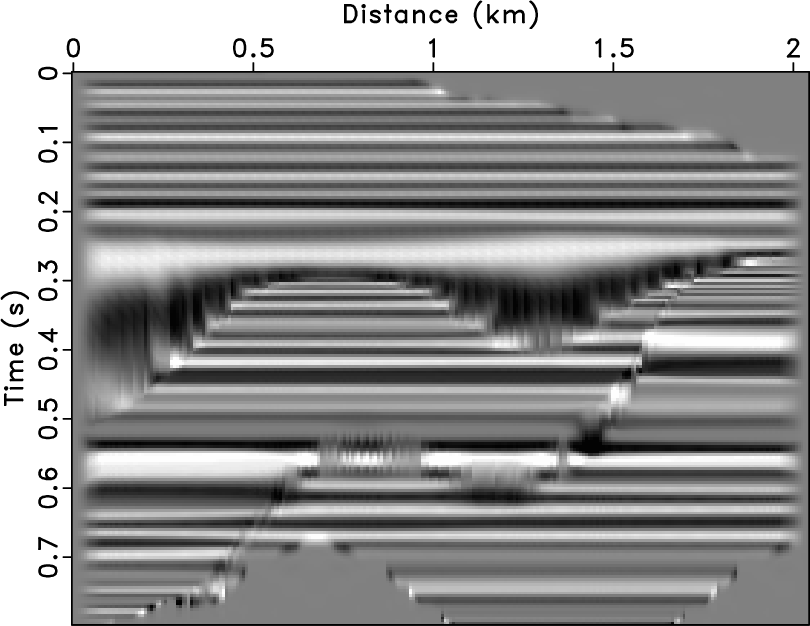
Figure 1 shows a synthetic image with several complex geologic structures. Local slopes corresponding to Figure 1 are shown in Figure 2, which are estimated by PWD. Figure 3a is the RT volume calculated by the predictive painting using local slopes in Figure 2. The reference trace of this RT volume is in the center of the image, which is marked as a vertical line in Figure 3a. This single reference RT volume is used to flatten the input seismic image (Figure 1) by unshifting each traces using the information it contains, since RT indicates how much a given trace is shifted with respect to the reference trace. The flattened image is shown in Figure 4a. Another RT volume with multiple references, shown in Figure 3b, is generated by selecting five reference traces and calculating the average of all estimated RT volumes. Figure 4b shows the corresponding flattened image. The comparison between two flattened seismic images (Figure 4a and 4b) indicates that the RT volume with only one reference trace does not necessarily have information about all seismic events since there are discontinuities such as faults and unconformities, while the RT volume computed with more reference traces contains more information.
|
|---|
|
sigmoid
Figure 1. Synthetic seismic image from Claerbout (2000). |
|
|
|
|---|
|
dip-pad
Figure 2. Local slopes estimated from Figure 1. |
|
|
|
|---|
|
pick-1,pick-5
Figure 3. RT estimated by predictive painting from Figure 1 using (a) a single reference trace and (b) multiple reference traces. |
|
|
|
|---|
|
flat-1,flat-5
Figure 4. Flattened images using RT volumes from (a) Figure 3a and (b) Figure 3b. |
|
|
|
|
|
|
Relative time seislet transform |