|
|
|
|
A parallel sweeping preconditioner for heterogeneous 3D Helmholtz equations |
One interpretation of radiation conditions is that they allow for the analysis of a finite portion of an infinite domain, as their purpose is to enforce the condition that waves propagate outwards and not reflect at the boundary of the truncated domain. This concept is crucial to understanding the Schur complement approximations that take place within the moving PML sweeping preconditioner which is reintroduced in this paper for the sake of completeness.
For the sake of simplicity, we will describe the preconditioner in the context
of a second-order finite-difference discretization over the unit cube,
with PML used to approximate a radiation boundary condition on the ![]() face
and homogeneous Dirichlet boundary conditions applied on all other boundaries
(an
face
and homogeneous Dirichlet boundary conditions applied on all other boundaries
(an ![]() cross-section is shown in Fig. 1).
If the domain is discretized into an
cross-section is shown in Fig. 1).
If the domain is discretized into an
![]() grid, then ordering the vertices in the grid such that
vertex
grid, then ordering the vertices in the grid such that
vertex
![]() is assigned index
is assigned index
![]() results in a block tridiagonal system of equations, say
results in a block tridiagonal system of equations, say
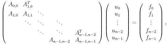 |
(2) |

|
|---|
|
plane-with-single-pml
Figure 1. An |
|
|
If we were to ignore the sparsity within each block, then the following
naïve factorization and solve algorithms would be appropriate for a
direct solver, where the application of ![]() implicitly makes use of the
factorization of
implicitly makes use of the
factorization of ![]() .
.
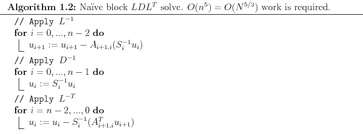
While the computational complexities of
Algs. 0.0.1 and 0.0.2 are significantly higher
than multifrontal algorithms
(21,27,12),
which have ![]() factorization complexity and
factorization complexity and
![]() solve complexity for regular three-dimensional meshes, they are the conceptual
starting points of the sweeping preconditioner.
solve complexity for regular three-dimensional meshes, they are the conceptual
starting points of the sweeping preconditioner.![]()
Suppose that we paused Alg. 0.0.1 after computing the ![]() 'th
Schur complement,
'th
Schur complement, ![]() , where the
, where the ![]() 'th
'th ![]() plane is in the
interior of the domain (i.e., it is not in a PML region).
Due to the ordering imposed on the degrees of freedom of the discretization,
the first
plane is in the
interior of the domain (i.e., it is not in a PML region).
Due to the ordering imposed on the degrees of freedom of the discretization,
the first ![]() Schur complements are equivalent to those that would have been
produced from applying Alg. 0.0.1 to an auxiliary problem
formed by placing a homogeneous Dirichlet boundary condition on the
Schur complements are equivalent to those that would have been
produced from applying Alg. 0.0.1 to an auxiliary problem
formed by placing a homogeneous Dirichlet boundary condition on the
![]() 'th
'th ![]() plane and ignoring all of the
successive planes (see the left half of Fig. 2).
While this observation does not immediately yield any computational savings,
it does allow for a qualitative description of the inverse of the
plane and ignoring all of the
successive planes (see the left half of Fig. 2).
While this observation does not immediately yield any computational savings,
it does allow for a qualitative description of the inverse of the ![]() 'th Schur
complement,
'th Schur
complement, ![]() : it is the restriction of the half-space Green's function
of the exact auxiliary problem onto the
: it is the restriction of the half-space Green's function
of the exact auxiliary problem onto the ![]() 'th
'th ![]() plane
(recall that PML can be interpreted as approximating the effect of a domain
extending to infinity).
plane
(recall that PML can be interpreted as approximating the effect of a domain
extending to infinity).
The main approximation made in the sweeping preconditioner can now be
succinctly described: since ![]() is a restricted half-space Green's
function which incorporates the velocity field of the first
is a restricted half-space Green's
function which incorporates the velocity field of the first ![]() planes, it is
natural to approximate it with another restricted half-space
Green's function which only takes into account the local velocity field,
i.e., by moving the PML next to the
planes, it is
natural to approximate it with another restricted half-space
Green's function which only takes into account the local velocity field,
i.e., by moving the PML next to the ![]() 'th plane (see the right half of
Fig. 2).
'th plane (see the right half of
Fig. 2).

|
|---|
|
auxiliary
Figure 2. (Left) A depiction of the portion of the domain involved in the computation of the Schur complement of an |
|
|
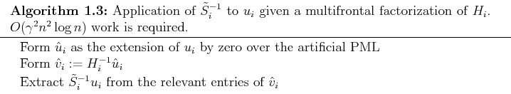
If we use
![]() to denote the number of grid points of PML as a
function of the frequency,
to denote the number of grid points of PML as a
function of the frequency, ![]() , then it is
important to recognize that the depth of the approximate auxiliary problems
in the
, then it is
important to recognize that the depth of the approximate auxiliary problems
in the ![]() direction is
direction is
![]() .
.![]() If the depth of the approximate auxiliary problems was
If the depth of the approximate auxiliary problems was ![]() , then
combining nested dissection with the multifrontal method over the regular
, then
combining nested dissection with the multifrontal method over the regular
![]() mesh would only require
mesh would only require ![]() work and
work and
![]() storage (21).
However, if the PML size is a slowly growing function of frequency, then
applying 2D nested dissection to the quasi-2D domain requires
storage (21).
However, if the PML size is a slowly growing function of frequency, then
applying 2D nested dissection to the quasi-2D domain requires
![]() work and
work and
![]() storage,
as the number of degrees of freedom in each front increases by a factor of
storage,
as the number of degrees of freedom in each front increases by a factor of
![]() and dense factorizations have cubic complexity.
and dense factorizations have cubic complexity.
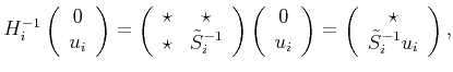
Let us denote the quasi-2D discretization of the local auxiliary problem for
the ![]() 'th plane as
'th plane as ![]() , and its corresponding approximation to the Schur
complement
, and its corresponding approximation to the Schur
complement ![]() as
as
![]() . Since
. Since
![]() is essentially a dense
matrix, it is advantageous to come up with
an abstract scheme for applying
is essentially a dense
matrix, it is advantageous to come up with
an abstract scheme for applying
![]() : Assuming that
: Assuming that ![]() was
ordered in a manner consistent with the
was
ordered in a manner consistent with the
![]() global ordering, the degrees of
freedom corresponding to the
global ordering, the degrees of
freedom corresponding to the ![]() 'th plane come last and we find that
'th plane come last and we find that
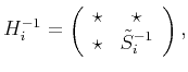 |
(3) |
 |
(4) |
From now on, we write ![]() to refer to the application of the
(approximate) inverse of the Schur complement for the
to refer to the application of the
(approximate) inverse of the Schur complement for the ![]() 'th plane.
'th plane.
There are two more points to discuss before defining the full serial algorithm.
The first is that, rather than performing an approximate ![]() factorization
using a discretization of
factorization
using a discretization of
![]() , the preconditioner is instead built
from a discretization of an artificially damped version of the Helmholtz
operator, say
, the preconditioner is instead built
from a discretization of an artificially damped version of the Helmholtz
operator, say
The second point is much easier to motivate: since the artificial PML in
each approximate auxiliary problem is of depth
![]() , processing
a single plane at a time would require processing
, processing
a single plane at a time would require processing ![]() subdomains with
subdomains with
![]() work each. Clearly, processing
work each. Clearly, processing ![]() planes at once
has the same asymptotic complexity as processing a single plane, and so
combining
planes at once
has the same asymptotic complexity as processing a single plane, and so
combining ![]() planes reduces the setup cost from
planes reduces the setup cost from
![]() to
to
![]() .
Similarly, the memory usage becomes
.
Similarly, the memory usage becomes
![]() instead of
instead of
![]() .
.![]() If we refer to these
sets of
If we refer to these
sets of ![]() contiguous planes as panels, which we label from
0
to
contiguous planes as panels, which we label from
0
to ![]() , where
, where
![]() , and correspondingly redefine
, and correspondingly redefine
![]() ,
, ![]() ,
, ![]() ,
, ![]() , and
, and ![]() ,
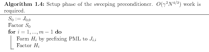
we have the following algorithm for setting up an approximate
block
,
we have the following algorithm for setting up an approximate
block ![]() factorization of the discrete artificially damped Helmholtz
operator:
factorization of the discrete artificially damped Helmholtz
operator:
Once the preconditioner is set up, it can be applied using a straightforward
modification of Alg. 0.0.2 which avoids
redundant solves by combining the application of ![]() and
and ![]() :
:
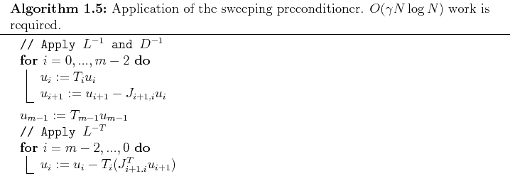
Given that the preconditioner can be set up with
![]() work,
and applied with
work,
and applied with
![]() work, it provides a near-linear scheme
for solving Helmholtz equations if only
work, it provides a near-linear scheme
for solving Helmholtz equations if only ![]() iterations are required for
convergence. The experiments in this paper seem to indicate that, as long as
the velocity model does not include a large cavity, the sweeping preconditioner
indeed only requires
iterations are required for
convergence. The experiments in this paper seem to indicate that, as long as
the velocity model does not include a large cavity, the sweeping preconditioner
indeed only requires ![]() iterations.
iterations.
Though this paper is focused on the parallel solution of Helmholtz equations, which are the time-harmonic form of acoustic wave equations, Tsuji et al. have shown that the moving PML sweeping preconditioner is equally effective for time-harmonic Maxwell's equations (39,38), and we believe that the same will hold true for time-harmonic linear elasticity. The rest of the paper will be presented in the context of the Helmholtz equation, but we emphasize that the parallelization should carry over to more general wave equations in a conceptually trivial way.
|
|
|
|
A parallel sweeping preconditioner for heterogeneous 3D Helmholtz equations |

![$\displaystyle \mathcal{J} \equiv \left[-\Delta - \frac{(\omega+i\alpha)^2}{c^2(x)}\right],$](img100.png)