|
|
|
|
Lowrank one-step wave extrapolation for reverse-time migration |
|
|---|
|
vel,wave2snap,diff,diff1
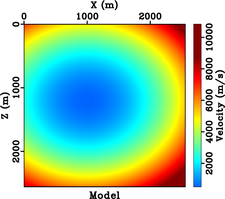
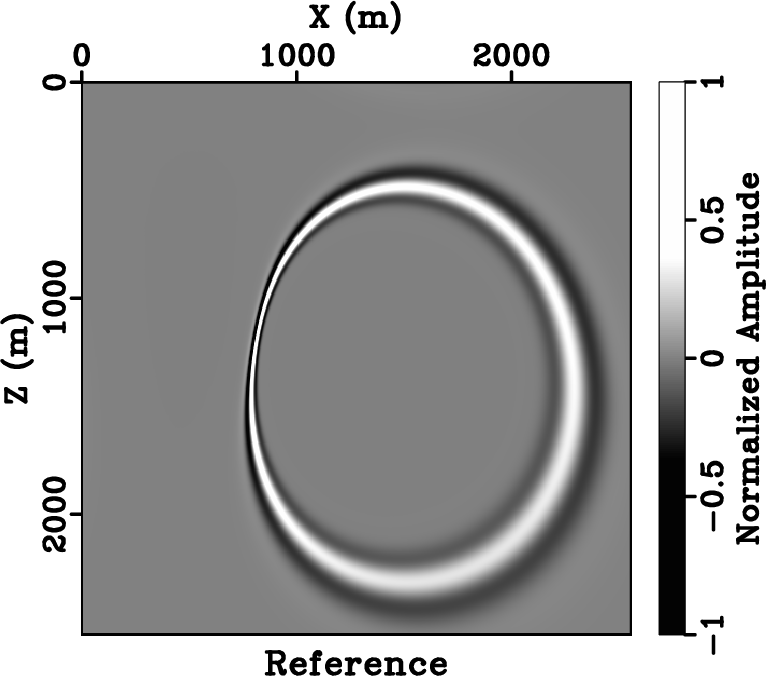
Figure 6. Wave propagation in a medium with large velocity variations. (a) Velocity model. (b) Reference wavefield propagated using |
|
|

|
|---|
|
compp,compp1
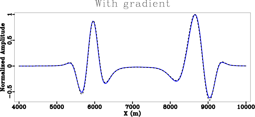
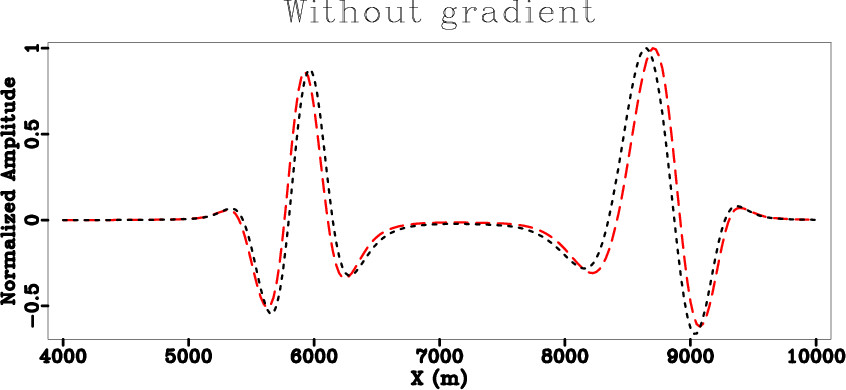
Figure 7. A slice through wavefields in Figure 6 at |
|
|
|
|---|
|
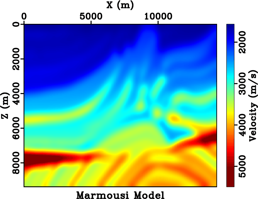
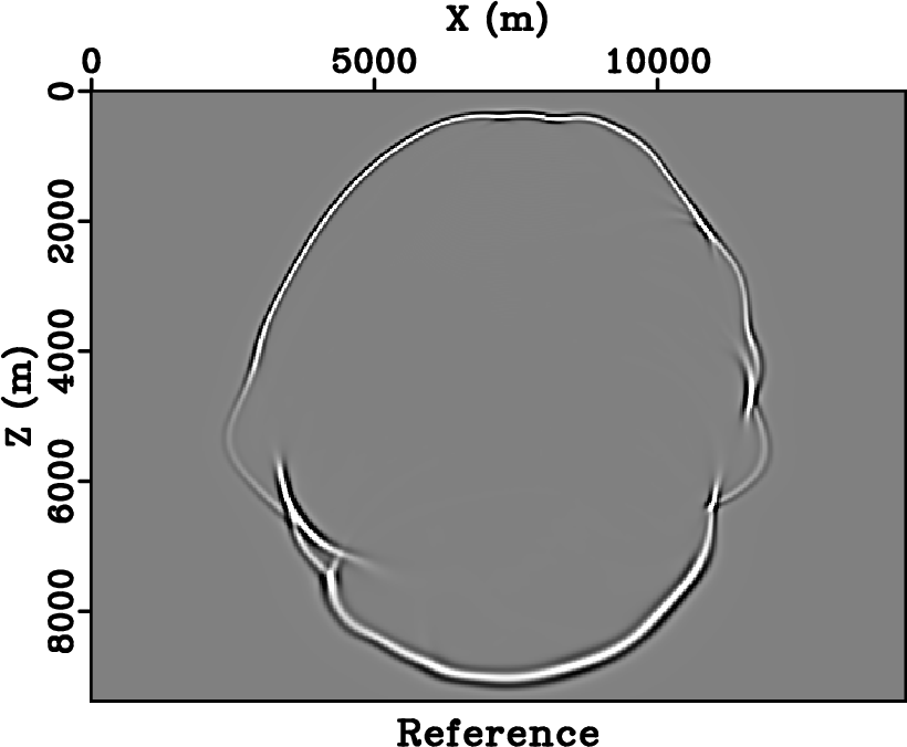
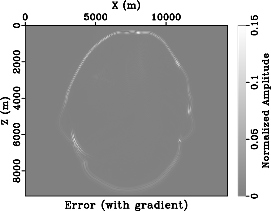
mvel,wave1snap-b,mdiff,mdiff1
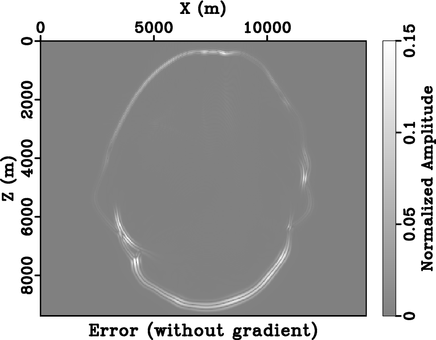
Figure 8. Wave propagation in a realistic velocity model. (a) Marmousi velocity model. (b) Reference wavefield propagated using |
|
|
|
|---|
|
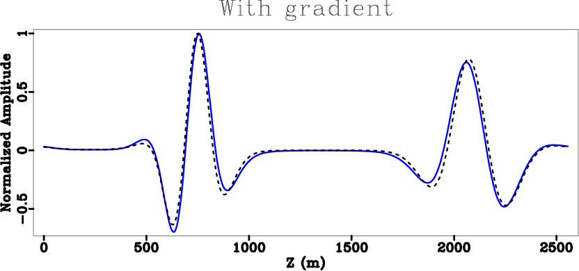
mcompp,mcompp1
Figure 9. A slice through wavefields in Figure 8 at |
|
|
To test if a more accurate wavefield can be obtained by using one-step extrapolation with equation 24, we first use a synthetic model with a smooth velocity distribution and large velocity variations (Figure 6a). We propagate a wavefield with the Ricker-wavelet source, using a time step of ![]() . The model is discretized on a
. The model is discretized on a
![]() grid with a spacing of
grid with a spacing of ![]() along both horizontal and vertical directions. The source is injected in the center of the model. Figure 6b shows the reference wavefield propagated using only the
along both horizontal and vertical directions. The source is injected in the center of the model. Figure 6b shows the reference wavefield propagated using only the ![]() term from equation 20, but with an exceedingly small time step (
term from equation 20, but with an exceedingly small time step (![]() ), so that the
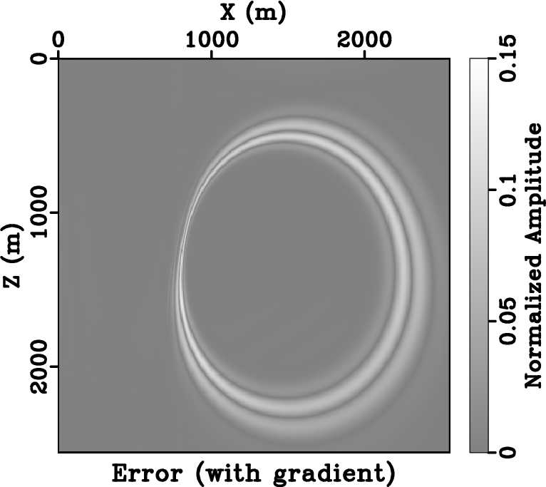
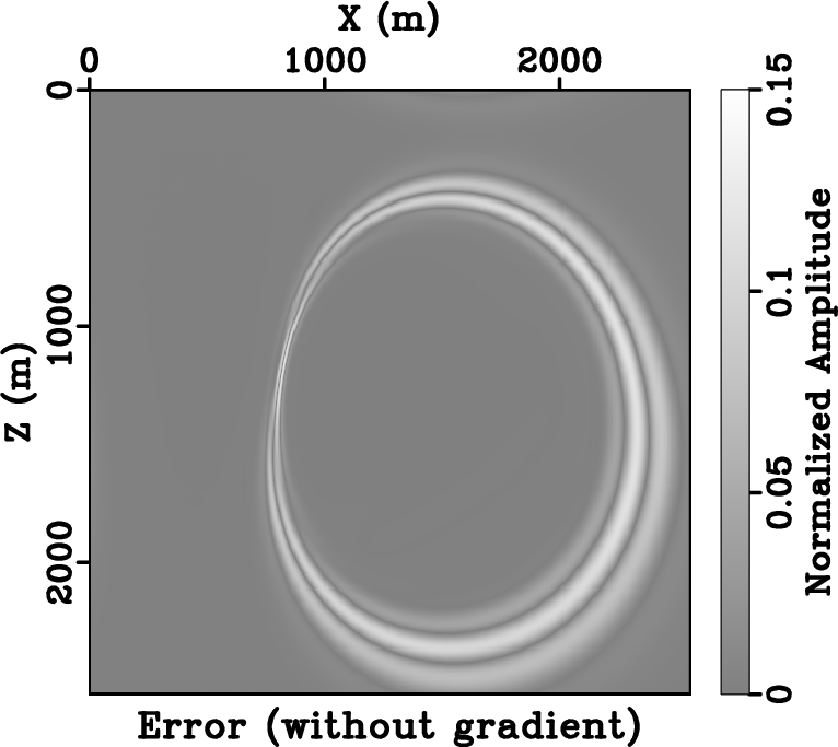
), so that the ![]() term is negligible and the wavefield can be treated as accurate. Figure 6c shows the difference between the reference wavefield and the wavefield propagated by equation 24 after normalization. Figure 6d shows the difference between the reference wavefield and the wavefield propagated without including the
term is negligible and the wavefield can be treated as accurate. Figure 6c shows the difference between the reference wavefield and the wavefield propagated by equation 24 after normalization. Figure 6d shows the difference between the reference wavefield and the wavefield propagated without including the ![]() term in the phase function, also after normalization. After including the velocity-gradient term, the error decreases significantly, and is caused mainly by small amplitude differences. On the other hand, the difference calculated without using the velocity-gradient term is due mostly to the shift in phase. This observation is further supported by Figure 7, which shows a comparison between traces extracted from the 2D wavefield snapshots at
term in the phase function, also after normalization. After including the velocity-gradient term, the error decreases significantly, and is caused mainly by small amplitude differences. On the other hand, the difference calculated without using the velocity-gradient term is due mostly to the shift in phase. This observation is further supported by Figure 7, which shows a comparison between traces extracted from the 2D wavefield snapshots at ![]() . The trace calculated using the velocity-gradient term aligns with the reference trace, whereas the trace calculated without including the velocity-gradient term has a noticeable shift in space relative to the reference trace. The shift increases with the degree of velocity variation.
. The trace calculated using the velocity-gradient term aligns with the reference trace, whereas the trace calculated without including the velocity-gradient term has a noticeable shift in space relative to the reference trace. The shift increases with the degree of velocity variation.
Next, we perform a similar experiment using a more complicated Marmousi velocity model (Figure 8a). The model is smoothed and discretized on a
![]() grid with a spacing of
grid with a spacing of ![]() . The reference wavefield is propagated using a time step size of
. The reference wavefield is propagated using a time step size of ![]() (Figure 8b). Figures 8c and 8d demonstrates the difference between the reference wavefield and the wavefields calculated using phase functions with and without the velocity gradient term. Figure 9 overlays the trace from the reference wavefield extracted at
(Figure 8b). Figures 8c and 8d demonstrates the difference between the reference wavefield and the wavefields calculated using phase functions with and without the velocity gradient term. Figure 9 overlays the trace from the reference wavefield extracted at ![]() with corresponding traces from the wavefields propagated using a larger time step size. The comparison shows that, even with moderate velocity variations but a relatively large time step size, the velocity gradient term can have a noticeable contribution to the phase accuracy.
with corresponding traces from the wavefields propagated using a larger time step size. The comparison shows that, even with moderate velocity variations but a relatively large time step size, the velocity gradient term can have a noticeable contribution to the phase accuracy.
In the remaining examples of this paper, the velocity gradient term was not included in the phase function for simplicity.
|
|
|
|
Lowrank one-step wave extrapolation for reverse-time migration |