|
 |
 |
 | Theory of interval traveltime parameter estimation in layered anisotropic media |  |
![[pdf]](icons/pdf.png) |
Next: Coefficients of traveltime expansion
Up: General formulas for traveltime
Previous: General formulas for traveltime
We can now substitute expressions for time derivative tensors from equations 21-24 into equations 5 and 6 and rewrite them as follows
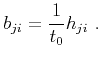
For convenience in subsequent derivation, we let elements of the matrix inverse of  be denoted as
 |
(27) |
Equations 25 and 26 represent the most general forms of the traveltime derivatives for pure-mode reflections in arbitrary anisotropic layered media.
Throughout the rest of this text, we continue to use the upper-case letters ( ,
,  , ...) to denote interval parameters. The lower-case letters (
 ,
,  , ...) are used to indicate effective values corresponding to the same quantities. In the case of effective values, the subscript refers to the effective value from the surface down to the bottom of the corresponding layer. Therefore, in this notation, we can denote the interval expression in equation 25 for the
  -th layer and the effective counterpart down to the
-th layer as
-th layer and the effective counterpart down to the
-th layer as  and
and  respectively.
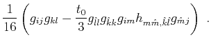
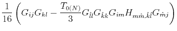
Let us first consider the second-order term in equation 27. In the case of multiple layers, there are direct accumulations of traveltime and offset as
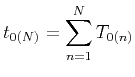 and and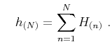 |
(28) |
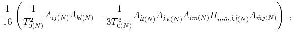
We can deduce
 |
(29) |
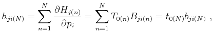
where  and
and  denote the vertical one-way traveltime and the inverse of interval matrix
in the
-th layer, and
denote the vertical one-way traveltime and the inverse of interval matrix
in the
-th layer, and  and
and  denote the effective values of the same two parameters at the bottom of the
  -th layer. Therefore, we can find the interval
  of the
-th layer from
of the
-th layer from
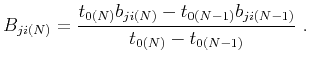 |
(30) |
Equation 30 is referred to as the generalized Dix equation (Tsvankin and Grechka, 2011). Applying matrix inversion to its result produces the second-order interval coefficients ( ), which are related to 3D NMO ellipse parameters. In the isotropic case, equation 30 reduces to classic Dix inversion (Dix, 1955).
We can now turn to equation 26 for the quartic coefficients and follow an analogous procedure. In this expression, only
 term needs to be considered because other terms can be simply related to
  . Equation 26 leads to
 |
(31) |
By substituting equations 25 and 27, we arrive at
 |
(32) |
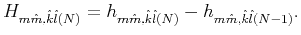
which can be used to find the interval
 in the
-th layer by a simple subtraction:
in the
-th layer by a simple subtraction:
 |
(33) |
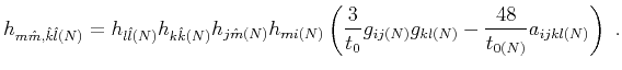
We can then compute the interval quartic coefficient
 in the
-th layer from the interval form of equation 26 given the interval value of equation 25 obtained from the generalized Dix equation (equation 30), as follows:
in the
-th layer from the interval form of equation 26 given the interval value of equation 25 obtained from the generalized Dix equation (equation 30), as follows:
where
 denotes the vertical one-way traveltime in the
-th layer. Thus, the second- and fourth-order interval coeffcients for the traveltime expansion can be found from equations 30 and 34 respectively, The exact expressions for the traveltime expansion coefficients in two particular cases of a horizontal stack of aligned orthorhombic layers and a horizontal stack of azimuthally rotated orthorhombic layers are detailed in the subsequent sections.
denotes the vertical one-way traveltime in the
-th layer. Thus, the second- and fourth-order interval coeffcients for the traveltime expansion can be found from equations 30 and 34 respectively, The exact expressions for the traveltime expansion coefficients in two particular cases of a horizontal stack of aligned orthorhombic layers and a horizontal stack of azimuthally rotated orthorhombic layers are detailed in the subsequent sections.
|
|
|
|
| Theory of interval traveltime parameter estimation in layered anisotropic media | |
|
Next: Coefficients of traveltime expansion
Up: General formulas for traveltime
Previous: General formulas for traveltime
2017-04-14