Field data test

We also test the workflow on a field data example collected at Teapot Dome. Figure 4 shows the input seismic section. It is a 2D line extracted from the original 3D data volume which has been converted from time to depth. The seismic image will be used to guide the interpolation of 11 density well logs scattered along the section, they have been tied to the seismic volume using automatic seismic-well tying technique (Wu and Caumon, 2016).

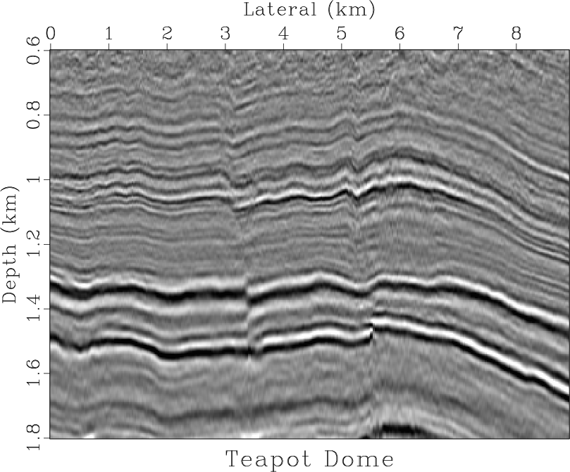
teapot
Figure 4. 2D seismic section from Teapot Dome data. The section is extracted from the original 3D data volume along a curve that passes through severa well locations.

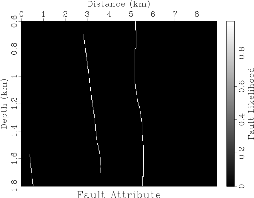
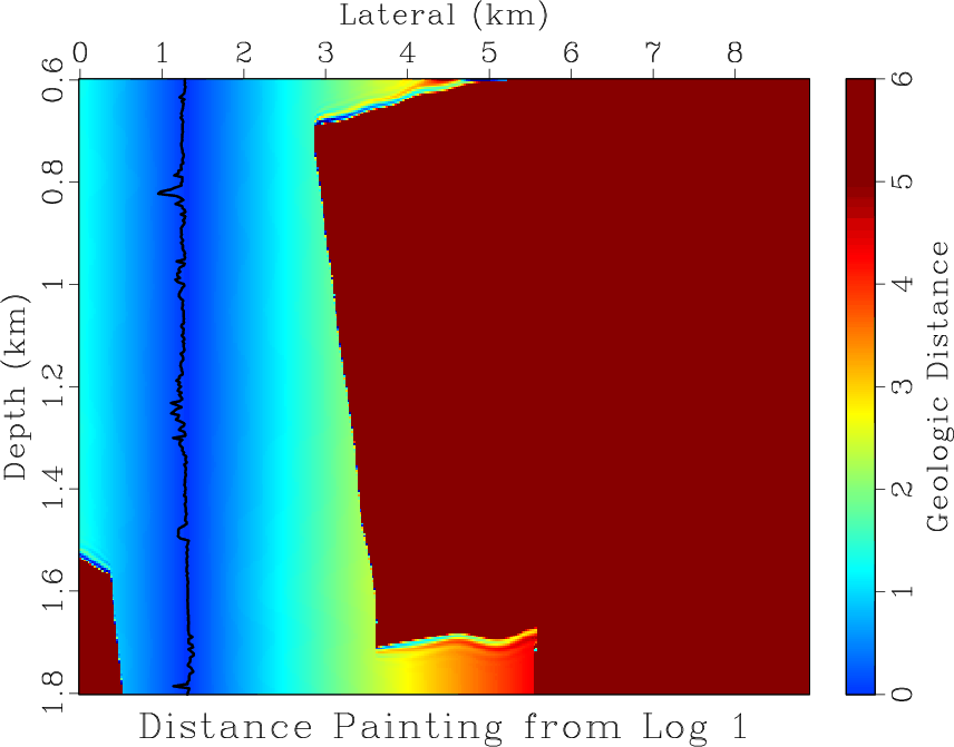
In this example, we use the method proposed by Wu (2017) based on structure-tensor to measure the fault attribute. It is shown in Figure 5 along with the geologic distance $\tilde d$ with regard to a reference well at about 12km. The image shows that at locations obscured by fault, geologic distance is magnified so that the RBF weight is expected to be suppressed.

fault,dist0
Figure 5. (a) fault likelihood attribute based on structure-tensor method; (b) the geologic distance $\tilde d$ computed according to the fault attribute.

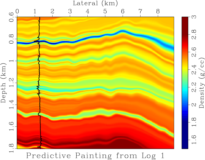
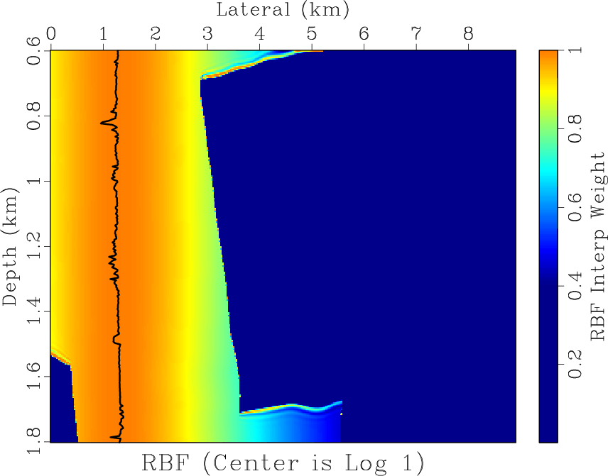
Figure 6 shows the predictive painting from the same well log and its corresponding RBF interpolation weight. Although painting prediction is conforming and smooth, in regions obscured by faults the prediction might be incorrect; however, the interpolation weight at such area will suppress the incorrect painting.

paint0,rbf0
Figure 6. (a) predictive painting from the well log located at about 12km laterally; (b) corresponding RBF weight, which will be used in interpolation later.

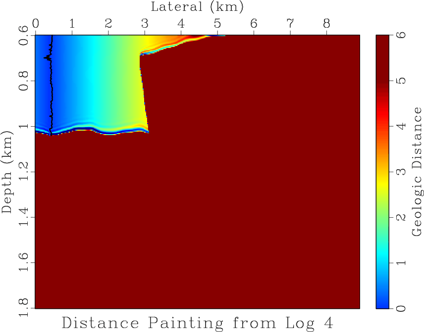
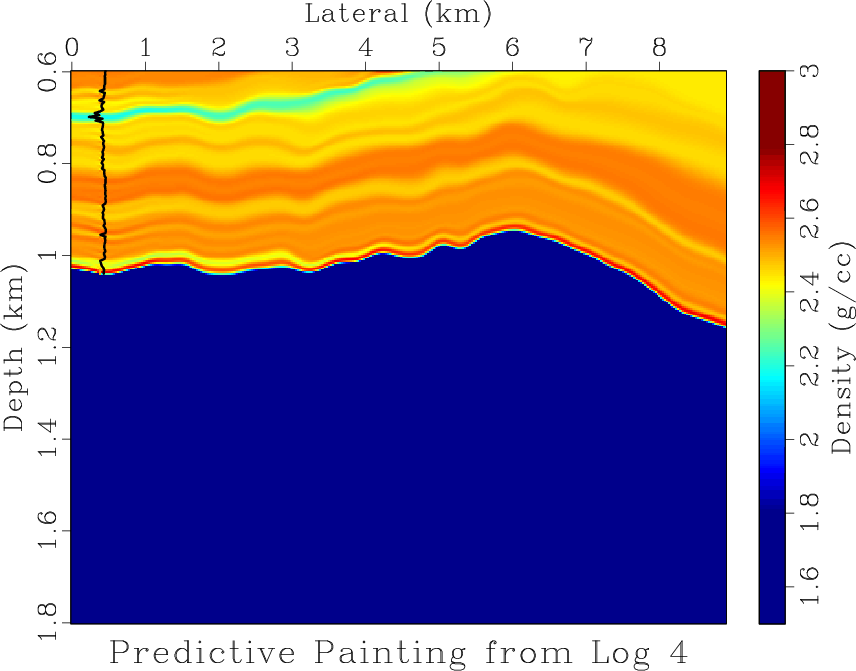
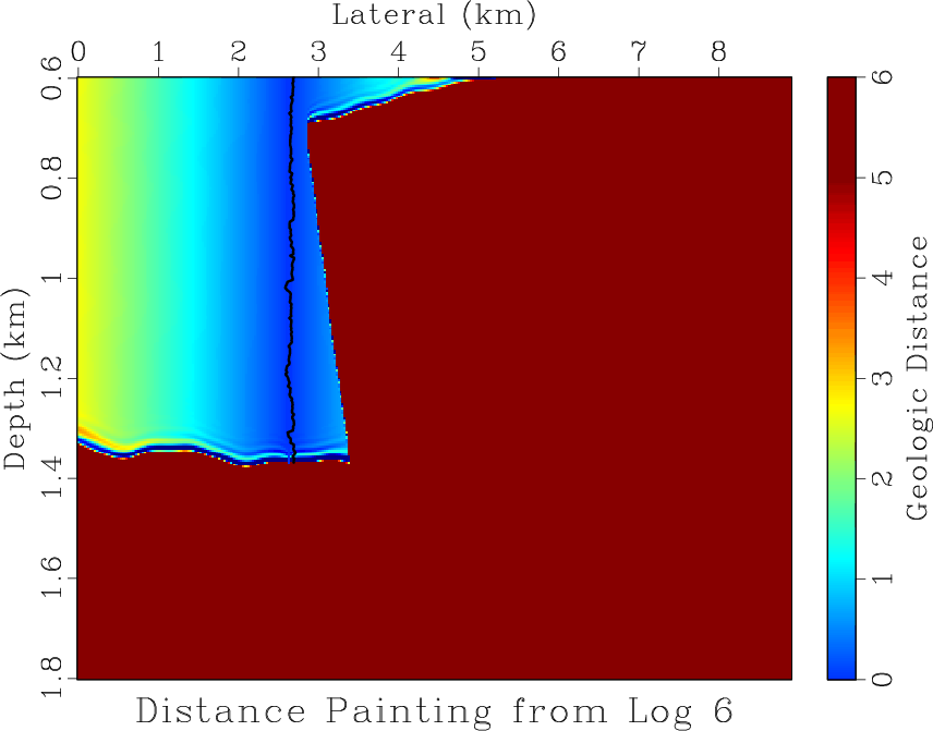
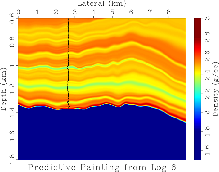
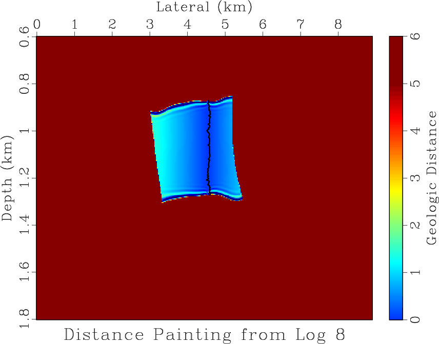
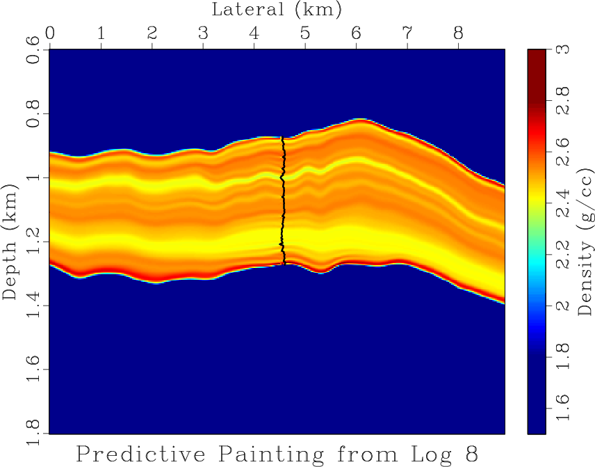
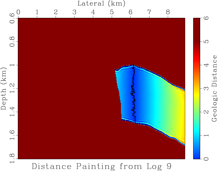
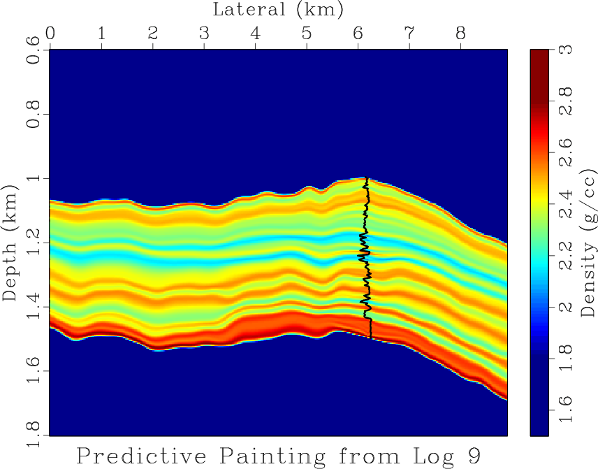
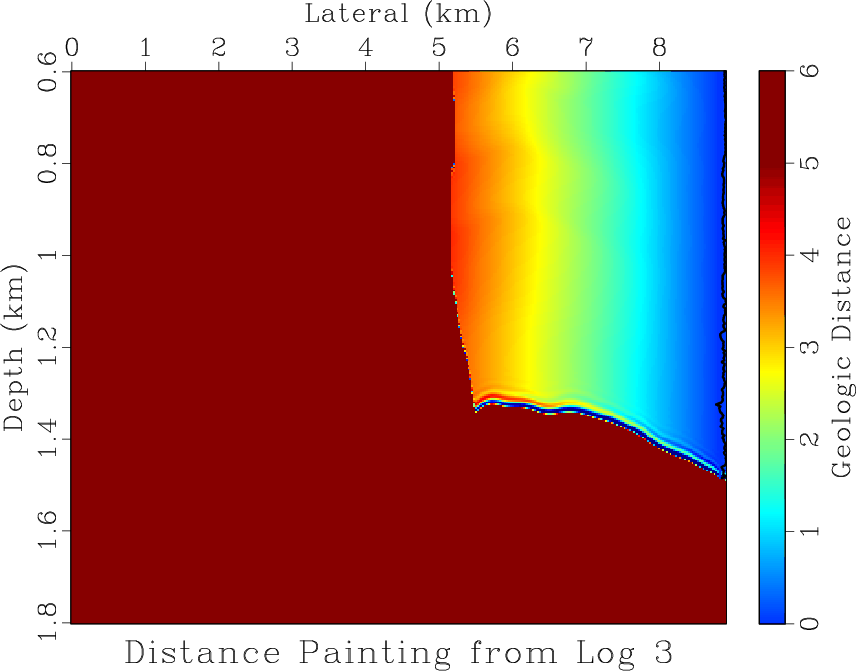
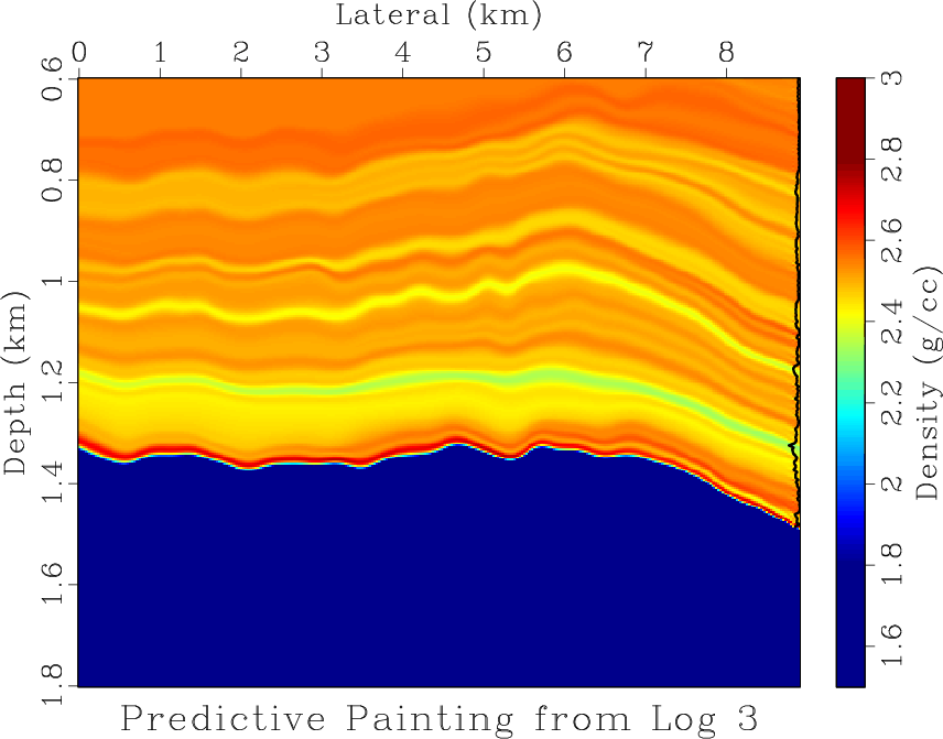
Figure 7 shows the geologic distances and corresponding predictive paintings from several other well logs.

dist3,paint3,dist5,paint5,dist7,paint7,dist8,paint8,dist2,paint2
Figure 7. (a,c,e,g,i) geologic distances $\tilde d$ and (b,d,f,h,j) the predictive paintings from corresponding well logs guided by the seismic image.

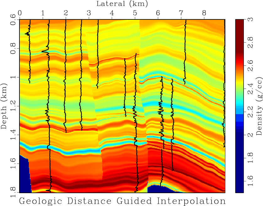
The final interpolation of eleven wells are shown in Figure 8.

interp-tpt
Figure 8. Interpolation result using 11 well logs on Teapot Dome data.