|
|
|
|
3D generalized nonhyperboloidal moveout approximation |
The choice of scheme for defining coefficient parameters can have an effect on the approximationa ccuracy. We chose to fit nine parameters (![]() ,
, ![]() , and
, and ![]() ) along the zero-offset ray. The remaining eight parameters are divided into six and two fitting equations. The former is from
) along the zero-offset ray. The remaining eight parameters are divided into six and two fitting equations. The former is from ![]() ,
, ![]() , and
, and ![]() along the
along the ![]() -axis and
-axis and ![]() ,
, ![]() , and
, and ![]() along the
along the ![]() - axis, while the latter is from
- axis, while the latter is from ![]() and
and ![]() along
along ![]() and
and ![]() . Another possible option is to consider
. Another possible option is to consider ![]() and the radial ray parameter
and the radial ray parameter
![]() , which would allow two fitting equations from all four directions and make the fitting scheme more symmetric. However, this approach degenerates even in the simple case of a homogeneous orthorhombic layer due to the similarity between
, which would allow two fitting equations from all four directions and make the fitting scheme more symmetric. However, this approach degenerates even in the simple case of a homogeneous orthorhombic layer due to the similarity between ![]() and
and ![]() directions caused by the orthorhombic symmetry. Therefore, we do not propose to use such scheme.
directions caused by the orthorhombic symmetry. Therefore, we do not propose to use such scheme.
Moreover, the selection of particular rays shot according to the proposed scheme also influences the accuracy level. This issue was originally pointed out by Fomel and Stovas (2010) and has been addressed by Hao and Stovas (2014) in the case of 3D HTI media. In our experiments, we observe that given the four rays at sufficiently far offsets, one can expect the proposed approximation to perform with sufficiently high accuracy for practical purposes with smaller errors closer to the chosen reference offsets.
Analogously to the 2D GMA of Fomel and Stovas (2010), the proposed approximation assumes that the traveltime at infinite offset behaves quadratically as
| (21) |
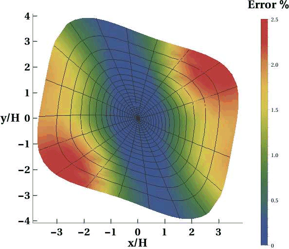
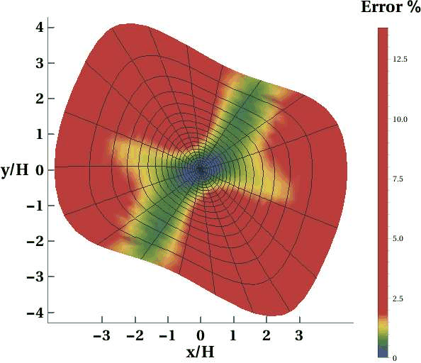
Even though the required number of parameters for the proposed approximation (seventeen) is high, this number is necessary for an accurate handling of anisotropy with complication from possible azimuthal rotation of the subsurface in 3D. Although other previously proposed approximations require fewer parameters, they may not produce equally accurate results. Figure 9 shows the results approximation of Xu et al. (2005) for the two models from last section, when 20% error is introduced in known azimuthal rotation. We can observe a significant decrease in accuracy especially in the layered case.
|
|---|
|
onelayerxuazi20,layeredxuazi503020
Figure 9. Error plots of the approximation by Xu et al. (2005) in a) the rotated homogeneous orthorhombic layer (Layer 1) and in b) the three-layer orthorhombic model with azimuthal rotation in sublayers plotted under similar color scales as the originals when 20% error is introduced in known azimuthal angles. One can observe significantly higher errors compared with the original ones in Figures 3c and 5c. |
|
|
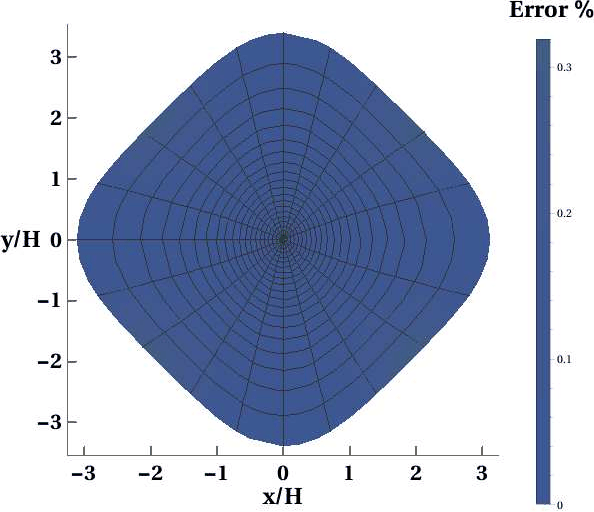
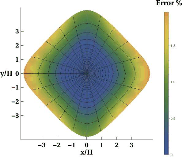
In the case of a single orthorhombic layer, the moveout approximation proposed in our earlier work (Sripanich and Fomel, 2015b), while requiring only six parameters, exhibits the same level of accuracy as the generalized approximation (Figure 10a). This indicates that the additional nonzero parameters in equation 1 can be captured by the relationship between anelliptic parameters in each symmetry plane (Sripanich et al., 2016; Sripanich and Fomel, 2015b). However, this approach may not be sufficiently accurate in a layered model (Figure 10b).
|
|---|
|
onelayerzone,layeredzone
Figure 10. Error plots of the approximation by Sripanich and Fomel (2015b) in a) the homogeneous orthorhombic layer (Layer 1) and in b) the aligned three-layer orthorhombic model. |
|
|
Provided that a reflection event can be accurately defined in a gather, the proposed 3D moveout approximation is suitable for anisotropic parameter estimation. One possible method for this application to real seismic data is time-warping (Burnett and Fomel, 2009; Casasanta and Fomel, 2011; Casasanta, 2011), which uses overdetermined least-squares parameter inversion based on local slope estimation and non-physical flattening by predictive painting (Fomel, 2010). This method enables in principles an estimation of all seventeen effective parameters in equation 1, which can then be inverted for interval values in a layer-stripping fashion (Sripanich and Fomel, 2016). In the presence of lateral heterogeneity, the results from such global inversion can be used as a initial model for more sophisticated inversion techniques.
|
|
|
|
3D generalized nonhyperboloidal moveout approximation |