|
|
|
|
Quantifying and correcting residual azimuthal anisotropic moveout in image gathers using dynamic time warping |
|
|---|
|
gather-250,stack-g-250
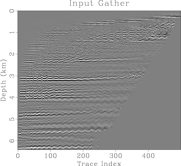
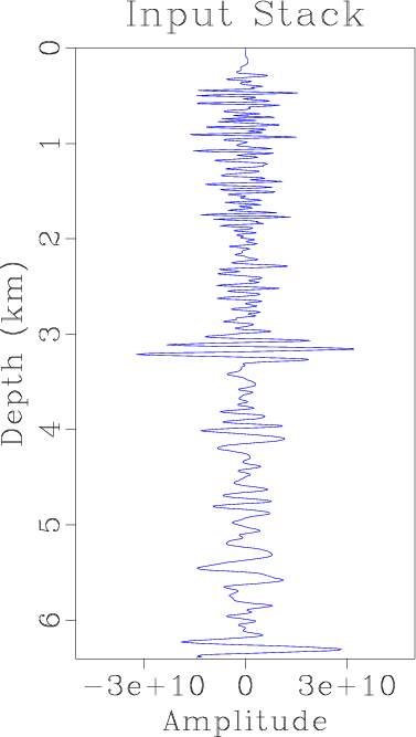
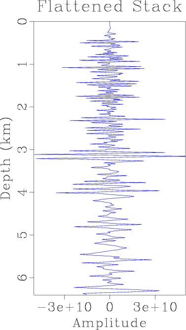
Figure 5. Gather flattening inputs: (a) common image gather with spiral structure; (b) the gather stack. |
|
|
We begin by flattening the gathers within the seismic volume by applying the same workflow as in our synthetic example. Shifts that best match traces within each gather to the gather's stack are calculated and then applied. Flattened gathers are stacked to generate an enhanced seismic image, called the flattened stack, and the shifts are integrated against a set of test functions according to equation 3 to determine the principal anisotropic axis and anisotropic intensity.
Figure 5a contains an example of a spiral gather from this survey, and Figure 5b plots its stack, or average trace value. Energy in the gather appears to have a periodic wiggle across the trace indexes. The periodic moveout is caused by horizontally transverse anisotropy, where the seismic velocity is faster in one azimuthal direction than the other. Some moveout with offset is also present, visible as a general trend upward to the right in some of the events within the gather. This residual moveout is due to the tomography process, where the VTI velocity model is initially generated on a fine grid, and then smoothed on a coarse grid. The smoothed coarse model is used to migrate data, which results in near and mid offset traces being properly aligned in the gather at the expense of some far offset traces.
|
|---|
|
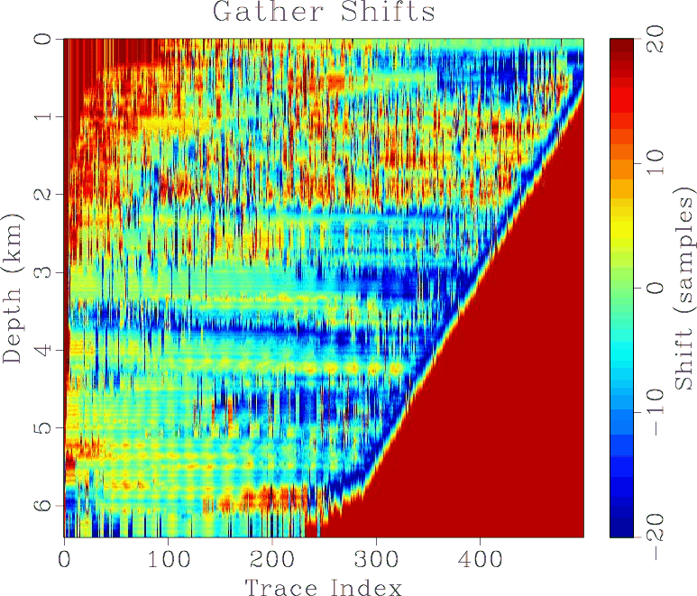
gather-shifts-250
Figure 6. The shifts that most closely match traces within the input gather in Figure 5a to the stack shown in Figure 5b. |
|
|
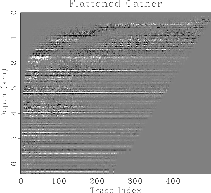
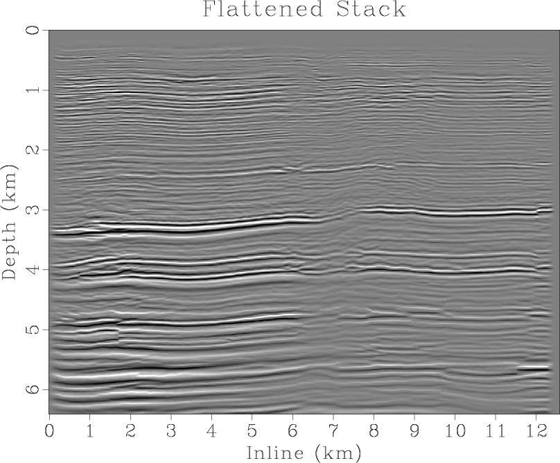
For each trace, we determine the shifts that best match that trace to the stack. These shifts are shown in Figure 6. Shifts are applied to traces in the input gather to create the flattened gather in Figure 7a and its stack in Figure 7b. Notice that the gather flattening process has corrected for the residual moveout with offset present in far offset traces as well as the periodic residual HTI moveout.
|
|---|
|
flat-gather-250,flat-stack-g-250
Figure 7. Gather flattening outputs: (a) flattened common image gather generated by applying the shifts in Figure 6 to the input gather in Figure 5a; (b) the flattened gather stack. |
|
|
Similar to the synthetic gather example, the azimuth of the principal axis is determined by finding the azimuthal anisotropy orientation ![]() in equation 1 that best fits the periodic portion of gather shifts. Then, the anisotropic intensity is determined. This process is illustrated in Figure 8.
in equation 1 that best fits the periodic portion of gather shifts. Then, the anisotropic intensity is determined. This process is illustrated in Figure 8.
|
|---|
|
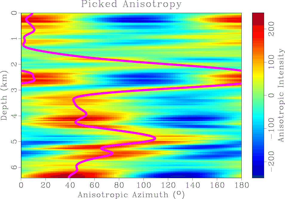
gather-anisotropic-pick
Figure 8. Illustration of determining the anisotropic parameters on this example gather based on the shifts in Figure 6. Background plots the value of equation 3 for different anisotropic azimuths. Solid fuchsia line plots the picked anisotropic azimuth which maximizes that equation at each time. The difference between the maximizing and minimizing value of equation 3 at each depth becomes the anisotropic intensity for this gather's spatial position. |
|
|
We repeat this process on all gathers within the seismic volume to enhance the stack, and determine anisotropic azimuth and intensity. Stacking in this example involves the average of all non-zero traces at each depth point within a gather, providing equal weight to non-zero samples.
|
|---|
|
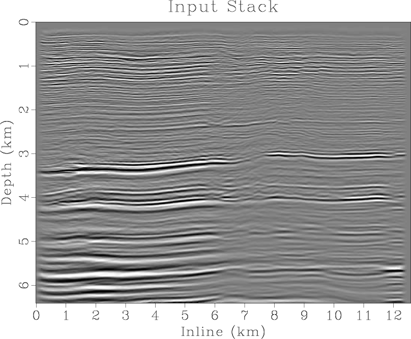
stack-inlin,flat-stack-inlin
Figure 9. Constant crossline slices of seismic volume visualizing: (a) the input stack; (b) the flattened stack. |
|
|
Figure 9a contains a constant crossline seismic image generated from stacking gathers prior to flattening. Figure 9b is the image that results from stacking the same gathers after flattening. Reflection events within the flattened stack generally appear sharper, more focused, and more coherent. Also note that events present in the flattened image have some corresponding signal in the input image - the process has not created new structure or shapes in the data.
|
|---|
|
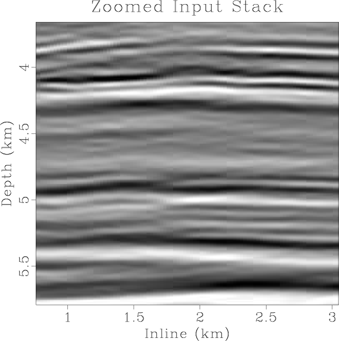
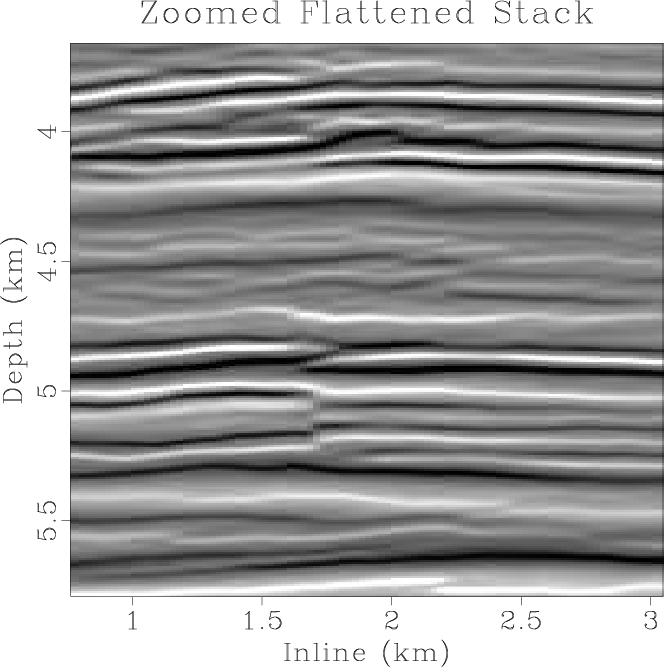
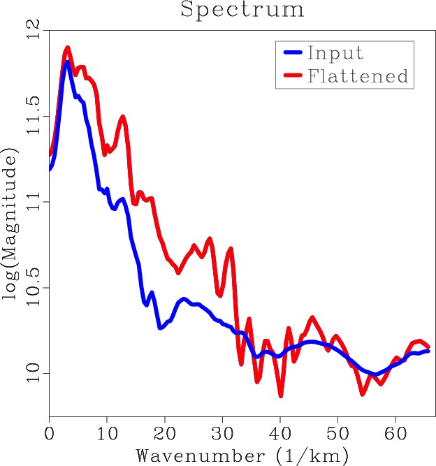
stack-inlin-zoom-1,flat-stack-inlin-zoom-1,spec-zm-1
Figure 10. Zoomed inline slices corresponding to: (a) the input stack; (b) the flattened stack; (c) visualizes the wavenumber spectrum of Figure 10a, the input stack, in blue and Figure 10b, the flattened stack, in red. |
|
|
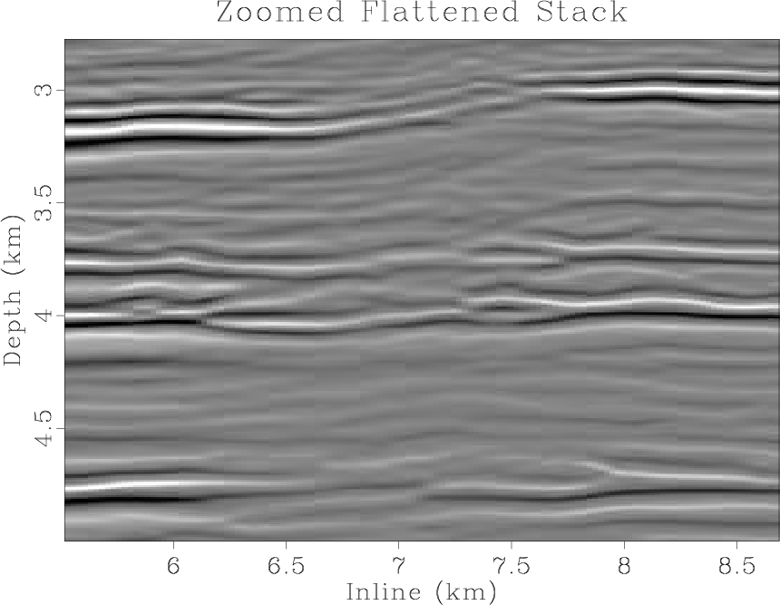
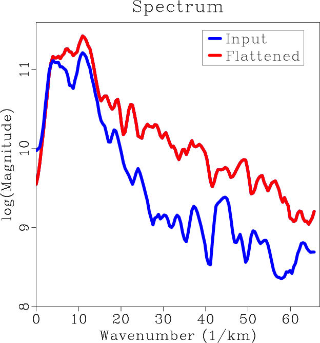
Figure 10a contains a first zoomed panel from the lower left portion of Figure 9a and Figure 10b contains the corresponding zoomed flattened stack from Figure 9b. Figures 10a and 10b contain zoomed inline slices of the input and flattened stacks, respectively. Notice how reflector discontinuities centered beneath 1.7 km are more apparent in the flattened stack. Reflection events appear sharper and more focused. Events in Figure 10b have some corresponding shapes in the image shown in Figure 10a, illustrating how the method amplifies already present structures. Figure 10c contains the wavenumber spectra of the two zoomed panels. The blue line corresponds to the input stack in Figure 10a and the red line corresponds to the flattened stack in Figure 10b. The red spectrum of the flattened stack contains more energy at higher wavenumbers than the blue spectrum of the input stack.
|
|---|
|
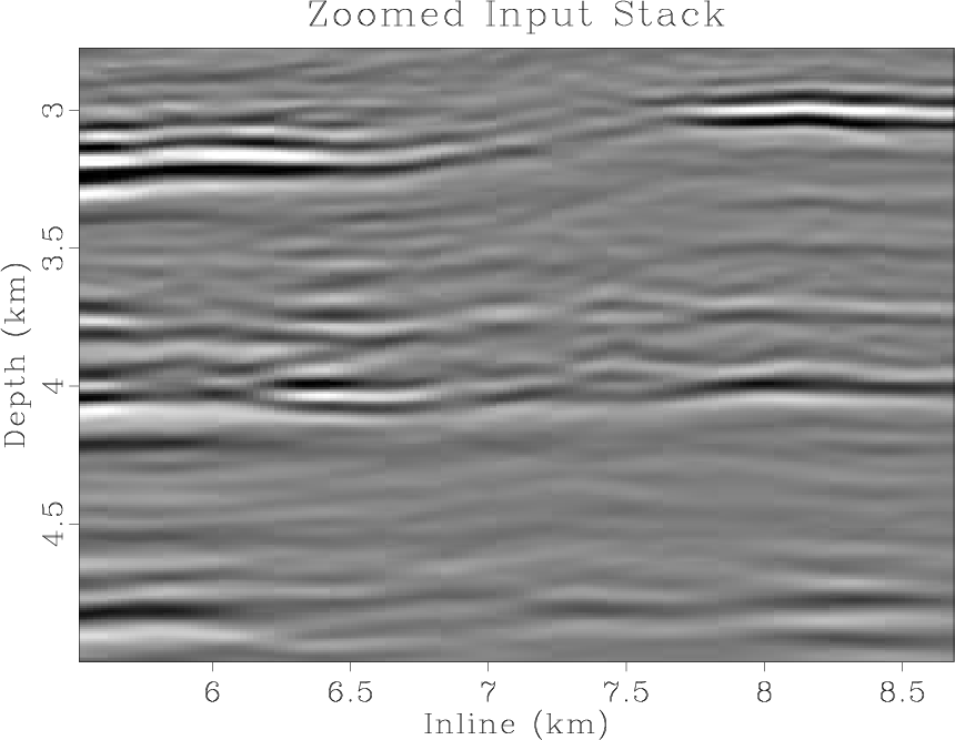
stack-inlin-zoom-2,flat-stack-inlin-zoom-2,spec-zm-2
Figure 11. A second set of zoomed panels originating from Figures 9a and 9b corresponding to: (a) the input stack; (b) the flattened stack; (c) visualizes the wavenumber spectrum of Figure 11a, the input stack, in blue and Figure 11b, the flattened stack, in red. |
|
|
Figure 11a contains a second zoomed panel from the central portion of Figure 9a and Figure 11b contains the corresponding zoomed panel of the flattened stack from Figure 9b. Events crossing the ``washed out'' portion of the image between 6.7-7.6 km are more coherent in the flattened stack, and an automatic picking algorithm would likely have an easier time following these more coherent horizons across the washout. Figure 11c contains the wavenumber spectrum of these two zoom panels. The blue line corresponds to Figure 11a and the red line corresponds to Figure 11b. As with Figure 10c, the spectrum of the flattened stack has greater energy at larger wavenumbers relative to the spectrum of the input stack spectrum and has increased bandwidth.
|
|---|
|
stack-zslice-2,flat-stack-zslice-2
Figure 12. First set of constant depth slices visualizing: (a) the input stack; (b) the flattened stack. |
|
|
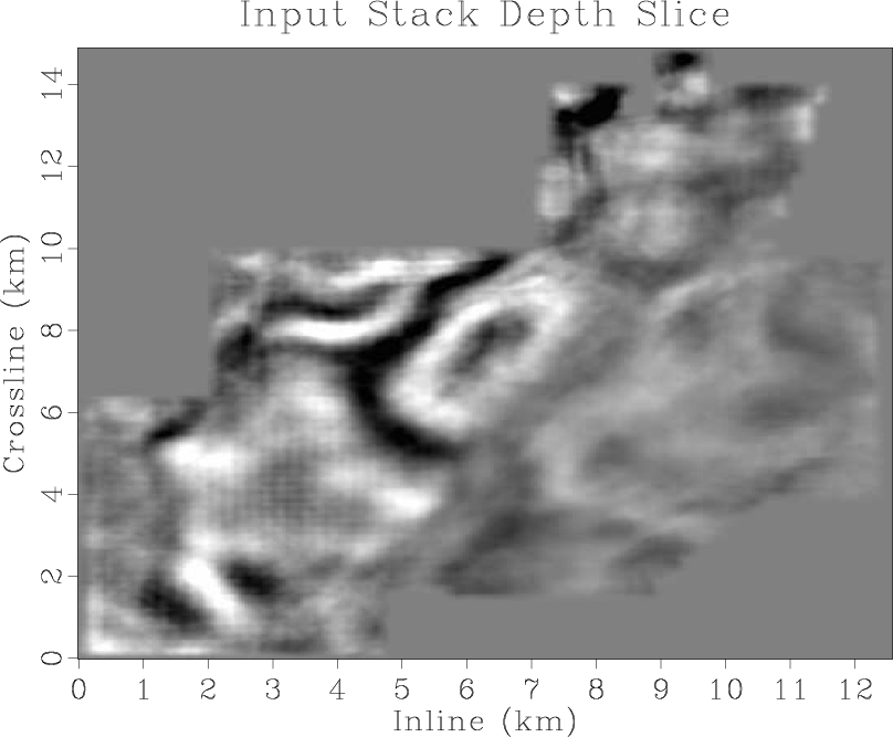
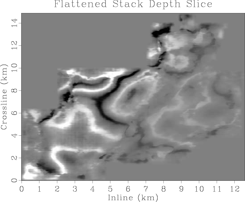
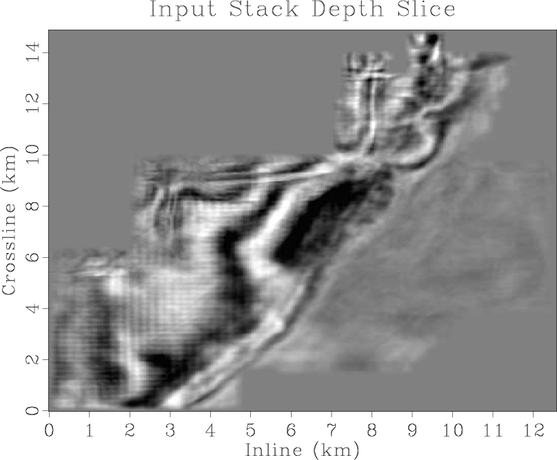
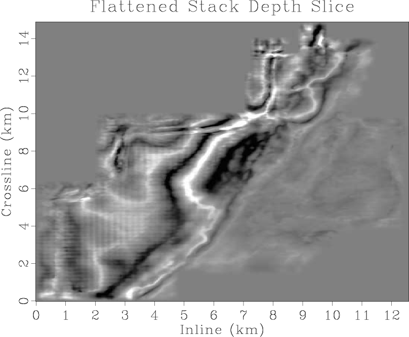
We visualize a first set of depth slices of the input and flattened stacks in Figures 12a and 12b, and zoomed sections of those slices in Figures 13a and 13b. Events in the flattened stack depth slices are significantly more coherent and focused than in the input stack slices, and the discontinuity caused by a fault running upward and to the right beginning at inline 3.5 km, crossline 0 km in Figures 12a and 12b is more easily visible in the flattened stack than in the input. Examining close-ups of the slices in Figures 13a and 13b, we see that features which appear as smudges or blurs in the input stack appear as coherent events in the flattened stack.
|
|---|
|
stack-zslice-zoom-2,flat-stack-zslice-zoom-2
Figure 13. Zoomed panels originating from Figures 12a and 12b corresponding to: (a) the input stack; (b) the flattened stack. |
|
|
|
|---|
|
stack-zslice-3,flat-stack-zslice-3
Figure 14. Second set of constant depth slices visualizing: (a) the input stack; (b) the flattened stack. |
|
|
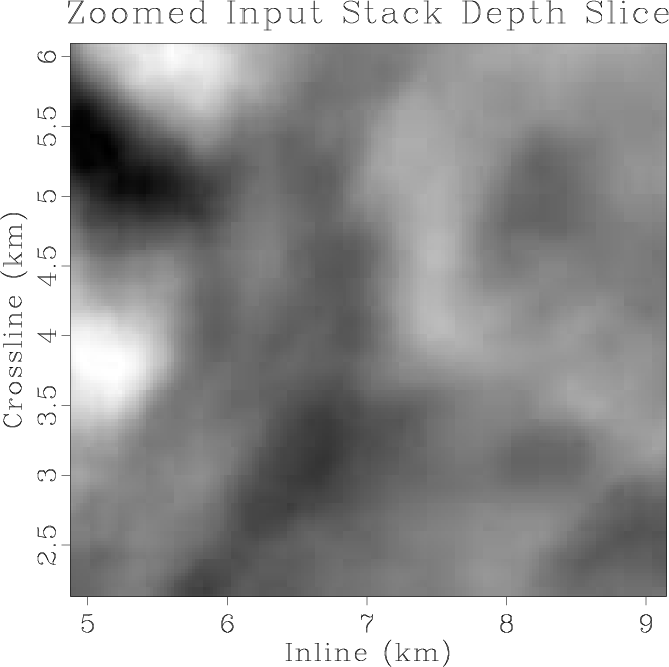
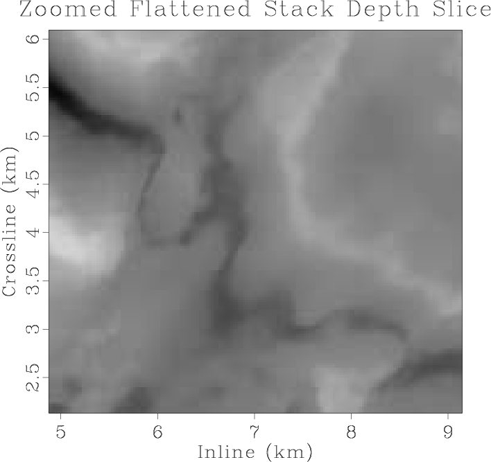
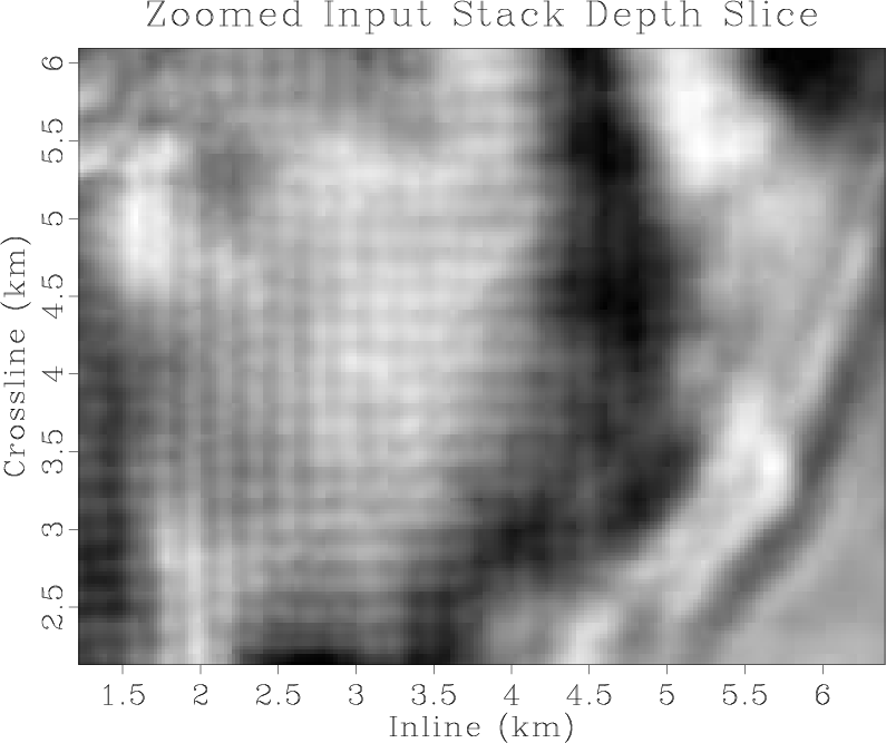
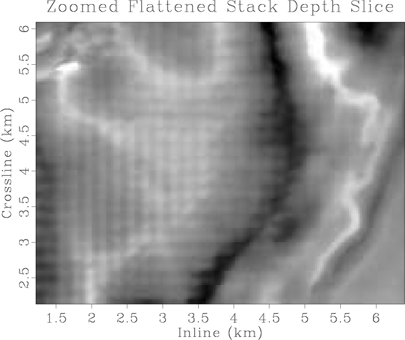
A second set of depth slices for input and flattened stacks are shown in Figures 14a and 14b. Again, events in the depth slices of the flattened stack are more coherent and focused than those of the input slice. Notice that a checkerboard artifact corresponding to the acquisition footprint is present for both the input and flattened slices in the lower left corner, highlighted in the zoomed depth slices of Figures 15a and 15b. This illustrates how the process of flattening does not create new shapes in the data, but rather aligns traces so they more closely match existing shapes. The process of gather flattening will not suppress coherent artifacts that are present in an image, as it assumes any coherent feature is signal.
|
|---|
|
stack-zslice-zoom-3,flat-stack-zslice-zoom-3
Figure 15. Zoomed panels originating from Figures 14a and 14b corresponding to: (a) the input stack; (b) the flattened stack. |
|
|
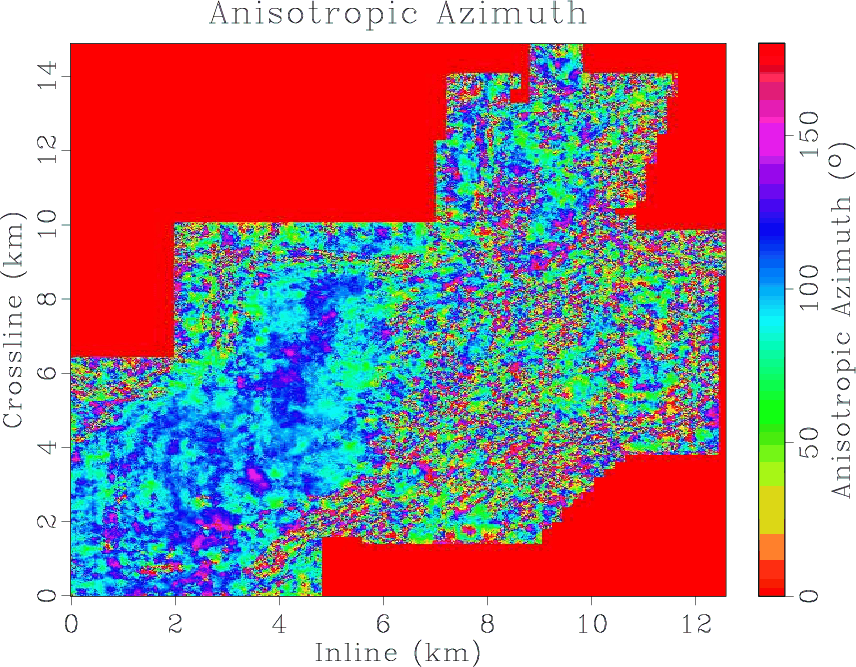
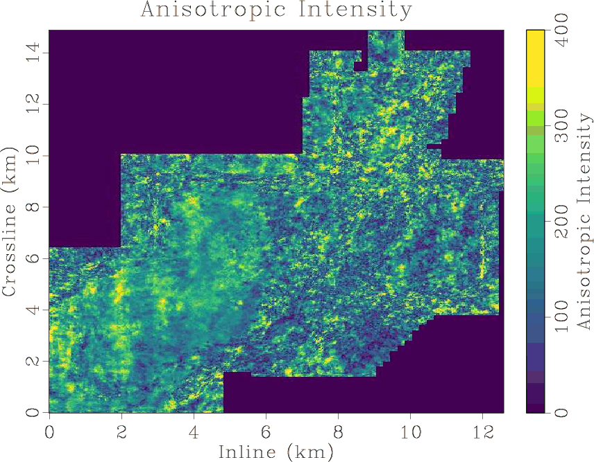
The anisotropic azimuth for the same depth slice as shown in Figures 14a and 14b is displayed in Figure 16a, while Figure 16b contains the anisotropic intensity for that depth slice. For both of the attributes, the region between 0-6 km inline and 0-9 km crossline has relatively consistent values. Here, anisotropic azimuth values mostly range between 90-130 degrees, and anisotropic intensity values do not vary as greatly as in other portions of the depth slice. This appears to be a relatively homogeneous portion of the slice, with relatively consistent anisotropic orientation and intensity. Presumably, this implies that a relatively consistent fracture network orientation and distribution exists there. Other areas of the slice, where the azimuth and intensity have greater variations, appear to indicate regions that may have a more chaotic distribution of fracture networks or other features causing elliptical HTI anisotropy. Results are consistent with proprietary log data acquired for wells in the study area.
|
|---|
|
azimuth-zslice,intensity-zslice
Figure 16. Anisotropic attribute visualization from the same depth slice as in Figures 14a and 14b: (a) the anisotropic azimuth, or the fastest azimuthal angle of seismic wave propagation; (b) the anisotropic intensity or relative difference between the velocities of the fastest and slowest azimuthal directions. |
|
|
|
|
|
|
Quantifying and correcting residual azimuthal anisotropic moveout in image gathers using dynamic time warping |