|
|
|
|
Quantifying and correcting residual azimuthal anisotropic moveout in image gathers using dynamic time warping |
We apply the concept of dynamic time warping (DTW) to flatten residual elliptical HTI moveout in image gathers generated using a processing workflow based on a VTI travel time approximation which did not consider azimuthal anisotropy. Ideally, the processing workflow would account for HTI anisotropy. However, that process is computationally expensive, motivating the approximation method presented here. We begin by first stacking an image gather by computing the average trace value. Misalignment of traces in the initial gather acts as a low pass filter, so this stack provides the low frequency gather information. For each trace in the gather we use DTW to determine the shifts that best align that trace with the initial low frequency gather stack, thus focusing events. This generates a function which may be used to warp constituent traces to correct for anisotropy and flatten the gather. Flattened gathers may then be stacked to create an enhanced image.
|
|---|
|
dtw-trace-m,dtw-trace-r
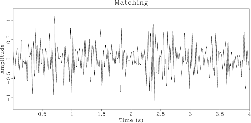
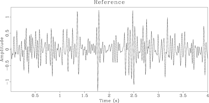
Figure 1. Input (a) matching and (b) reference traces used in DTW illustration reproduced from Hale (2013). Both traces are generated by convolving a reflectivity model with a 20 Hz Ricker wavelet and adding bandpassed noise. Applying a set of sinusoidal shifts with a maximum amplitude of 20 samples to the reflectivity used to generate the matching trace creates the reflectivity used to generate the reference trace. |
|
|
|
|---|
|
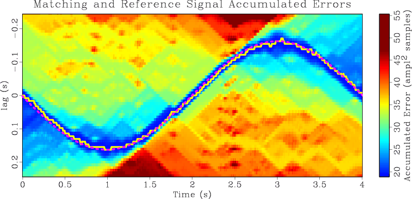
dtw-error,dtw-accum-sh
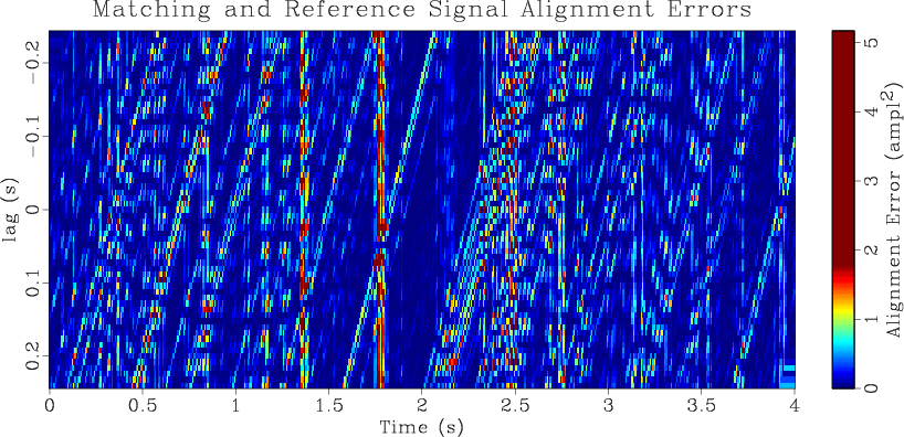
Figure 2. DTW illustration reproduced from Hale (2013): (a) Alignment errors resulting from the difference between the reference and matching trace when the reference trace is shifted by various lags; (b) Accumulated errors resulting from a symmetric error accumulation over the top panel subject to strain limitations. Solid yellow line plots the DTW shifts calculated through strain limited backtracking of the accumulated errors. Dotted fuchsia line plots the ideal shifts. |
|
|
Our gather flattening workflow is based on the use of dynamic time warping to match pairs of seismic signals, so we first illustrate the function of DTW by reproducing an example featured in Hale (2013). That paper provides a mathematical treatment of the DTW process as well as useful pseudocodes and advice for a successful implementation. We begin with a synthetic reflectivity section containing ![]()
![]() ms samples and apply sinusoidal shifts with 20 samples maximum amplitude to generate a shifted reflectivity model. Both reflectivity models are convolved with a 20 Hz Ricker wavelet and then bandpassed noise is added to create two synthetic traces. The trace resulting from the convolution of the wavelet with the initial reflectivity model is called the matching trace and is shown in Figure 1a. The trace resulting from the convolution of the wavelet with the shifted reflectivity is called the reference trace and is shown in Figure 1b.
ms samples and apply sinusoidal shifts with 20 samples maximum amplitude to generate a shifted reflectivity model. Both reflectivity models are convolved with a 20 Hz Ricker wavelet and then bandpassed noise is added to create two synthetic traces. The trace resulting from the convolution of the wavelet with the initial reflectivity model is called the matching trace and is shown in Figure 1a. The trace resulting from the convolution of the wavelet with the shifted reflectivity is called the reference trace and is shown in Figure 1b.
Alignment errors, shown in Figure 2a, are determined by computing the difference between the matching and reference signals at each point in the traces after shifting the matching trace by a set of lags, shown as the vertical coordinate. The sinusoidal path through the alignment errors panel defining the shifts is visible but difficult to follow. To make the path more discernible we accumulate over the alignment errors, shown in Figure 2b. This involves starting on the left of the alignment errors panel, and for each lag in the initial alignment errors trace, selecting the lag in the next trace sample with minimum error subject to a strain limitation of ![]() , meaning that the shifts may change by a maximum of one sample over five trace samples. The minimal permissible error of that next trace is added to the error of the previous lag, leading to the term ``accumulation''. These accumulated errors are written to the lag index in that subsequent trace, and the process is repeated, moving across the alignment errors panel to create the accumulated errors panel, Figure 2b. To remove the bias of general increase to the right in the accumulated errors panel, we accumulate from left to right and then from right to left. Accumulation both smooths the alignment errors and makes the optimal path more apparent, forming a blue ``valley''.
, meaning that the shifts may change by a maximum of one sample over five trace samples. The minimal permissible error of that next trace is added to the error of the previous lag, leading to the term ``accumulation''. These accumulated errors are written to the lag index in that subsequent trace, and the process is repeated, moving across the alignment errors panel to create the accumulated errors panel, Figure 2b. To remove the bias of general increase to the right in the accumulated errors panel, we accumulate from left to right and then from right to left. Accumulation both smooths the alignment errors and makes the optimal path more apparent, forming a blue ``valley''.
To compute the minimizing shifts we perform backtracking. To begin, we select the shift corresponding to the lag with the minimal accumulated error in the far right trace of Figure 2b. With this shift established we work backwards, picking the preceding permissible shift subject to the established strain limitations whose accumulated error value is minimal. This generates the set of shifts plotted in yellow in Figure 2b. Ideal shifts are plotted in dashed fuchsia, and have good agreement with the calculated shifts. Applying the calculated shifts to the matching trace will warp its values so that they match the reference trace as closely as permissible.
Returning to the gather domain, suppose we average the traces within a gather to make a stack and then use DTW to match each constituent trace within that gather to the stack. This matching operation provides a set of shifts for each trace which best align that trace to the stack. Note that although only integer shifts are considered, these shifts may vary with the trace sample index. In the presence of a HTI media, the residual moveout within a gather, and hence the flattening shifts, may be considered as periodic over
![]() where
where ![]() is gather azimuth and
is gather azimuth and ![]() is the anisotropic fast axis orientation (Grechka and Tsvankin, 1998; Mallick et al., 1997). We note that if our migration does not take this type of anisotropy into account, traces in a gather along the fast axis direction will be migrated with too low a velocity, and thus appear at a smaller time or shallower depth value than the stack, which represents an average trace for the gather. Similarly, traces along the slow axis direction will be migrated with too high a velocity and will appear at a greater time or depth than the stack. Based on how the shifts are defined in DTW, negative shifts ``push'' data downward in the positive time or depth direction, while positive shifts ``pull'' it upward in the negative time or depth direction. Thus, the most negative shift will be aligned with the fast axis of anisotropy and the most positive shift will be aligned with the slow anisotropic axis. If we assume that all other velocity and anisotropy corrections have been completed successfully, leaving only the component of moveout associated with elliptical HTI anisotropy, and that the anisotropic dependence on inclination
is the anisotropic fast axis orientation (Grechka and Tsvankin, 1998; Mallick et al., 1997). We note that if our migration does not take this type of anisotropy into account, traces in a gather along the fast axis direction will be migrated with too low a velocity, and thus appear at a smaller time or shallower depth value than the stack, which represents an average trace for the gather. Similarly, traces along the slow axis direction will be migrated with too high a velocity and will appear at a greater time or depth than the stack. Based on how the shifts are defined in DTW, negative shifts ``push'' data downward in the positive time or depth direction, while positive shifts ``pull'' it upward in the negative time or depth direction. Thus, the most negative shift will be aligned with the fast axis of anisotropy and the most positive shift will be aligned with the slow anisotropic axis. If we assume that all other velocity and anisotropy corrections have been completed successfully, leaving only the component of moveout associated with elliptical HTI anisotropy, and that the anisotropic dependence on inclination ![]() is independent of azimuth, we may model our gather shifts as
is independent of azimuth, we may model our gather shifts as
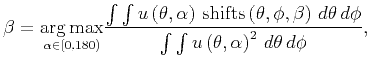
We solve for phase argument ![]() by integrating the test functions
by integrating the test functions
![]() against the shifts to interrogate the data for the correct phase argument. If we chose our test functions to have the form
against the shifts to interrogate the data for the correct phase argument. If we chose our test functions to have the form
This method works for gathers with arbitrary sampling in ![]() and
and ![]() , provided sufficient distribution of
, provided sufficient distribution of ![]() samples to avoid aliasing. Based on the way the method was constructed, it also works for gathers sampled in offset rather than inclination, and traces sampled in either depth or time. If the shifts have a strong positive or negative bias it may be beneficial to correct them so the summation of shifts over the trace index for each time or depth within a gather is equal to zero.
samples to avoid aliasing. Based on the way the method was constructed, it also works for gathers sampled in offset rather than inclination, and traces sampled in either depth or time. If the shifts have a strong positive or negative bias it may be beneficial to correct them so the summation of shifts over the trace index for each time or depth within a gather is equal to zero.
|
|
|
|
Quantifying and correcting residual azimuthal anisotropic moveout in image gathers using dynamic time warping |