|
|
|
|
Simultaneous denoising and reconstruction of 5D seismic data via damped rank-reduction method |
Next: Conclusion Up: GJI - Chen et Previous: Damped rank-reduction method for
|
|
|
|
Simultaneous denoising and reconstruction of 5D seismic data via damped rank-reduction method |
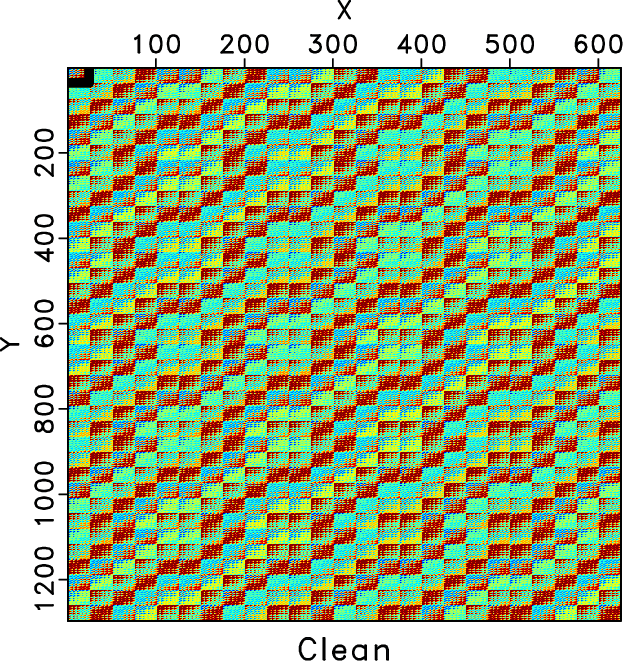
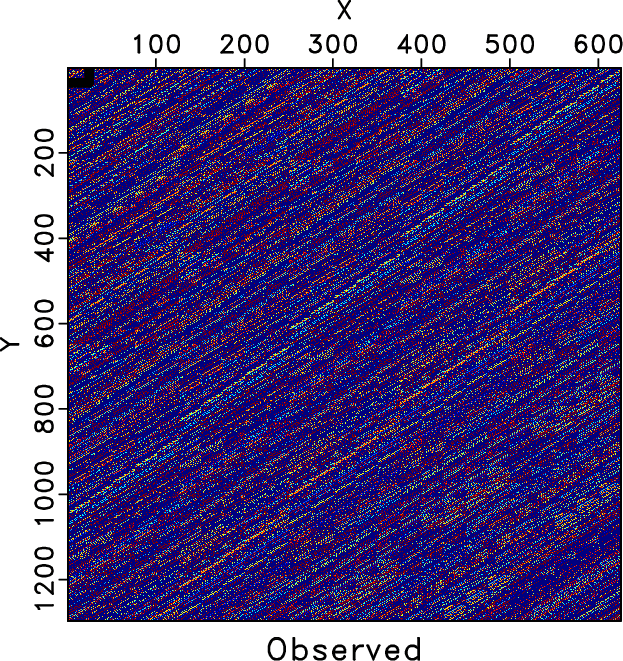
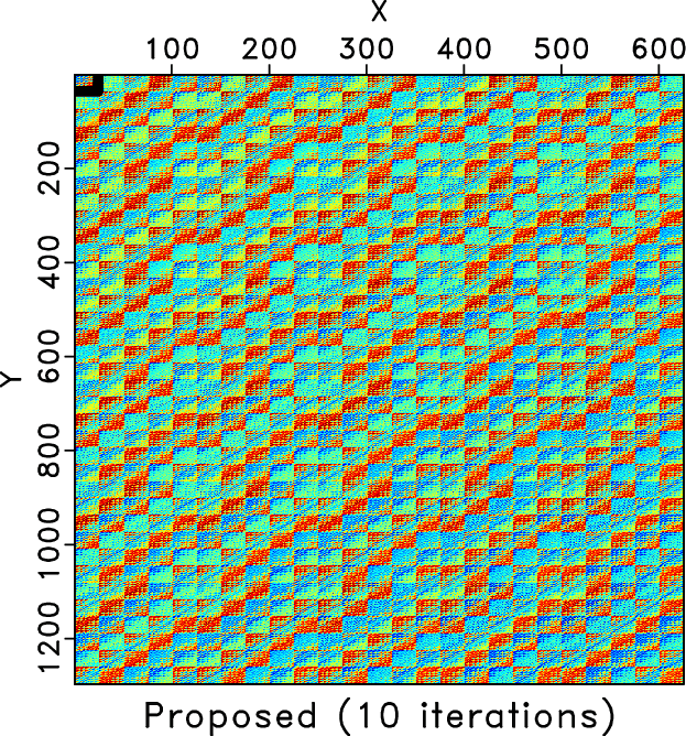
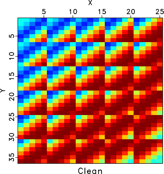
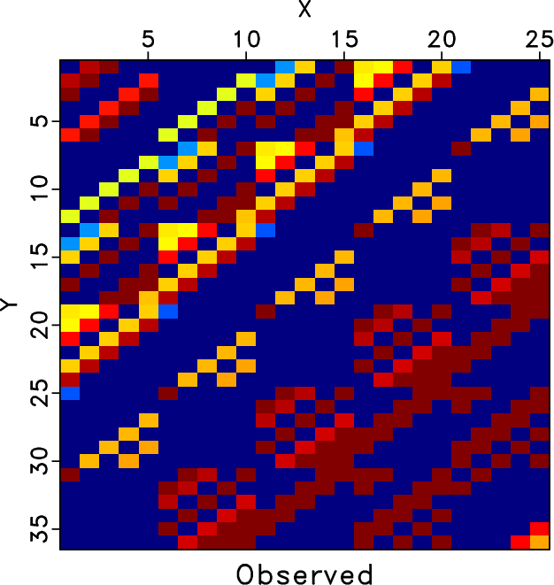
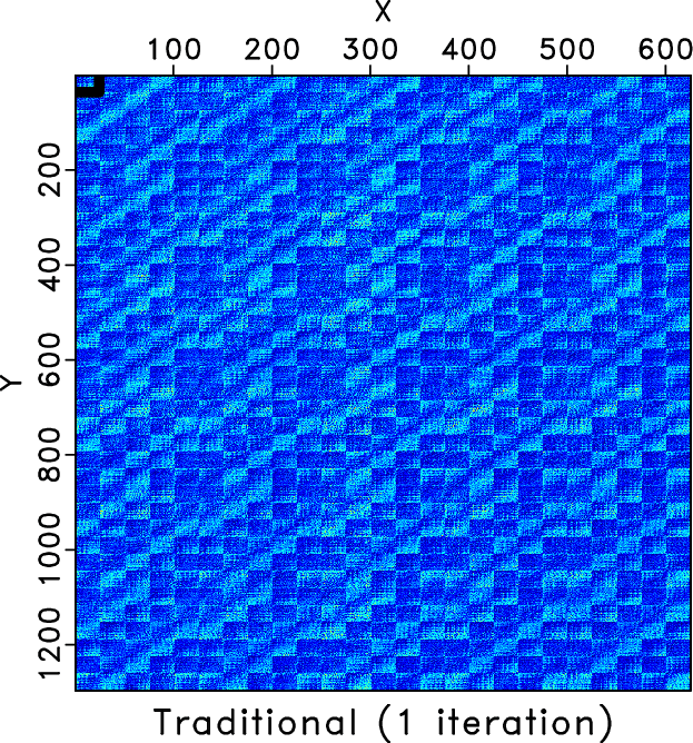
In order to show how the rank-reduced block Hankel matrix looks like and to more intuitively demonstrate the influence of the introduced damping operator to the target level-four block Hankel matrix in the first 5D seismic data example, we plot the 26 Hz block Hankel matrix for different cases in Figures 6, 7, and 8. Figure 6a shows the 26 Hz block Hankel matrix for the clean data. Figure 6b shows the 26 Hz block Hankel matrix for the observed data, which is very different from that of the true data due to the 70% missing traces. Figure 6c shows rank-reduced block Hankel matrix via the traditional TSVD after 10 iterations. The rank-reduced block Hankel matrix via the damped TSVD is shown in Figure 6d. Figures 6c and 6d are both close to the true block Hankel matrix and are very similar to each other. If we look carefully or zoom in the figure a bit, we can see that the block Hankel matrix via the traditional TSVD is much rougher than the Hankel matrix via the damped TSVD. Considering that each subfigure in Figure 6 is a 1296![]() 625 matrix, which contains a lot of information, we zoom one block Hankel matrix, as highlighted by the black frame boxes in Figure 6 and make a more detailed comparison in Figure 7. Figure 7 clearly shows that the rank-reduced block Hankel matrix via traditional TSVD still contains some artifacts, especially on the right bottom side, when compared with the true block Hankel matrix. The block Hankel matrix from the proposed approach is, however, much smoother, and closer to the true block Hankel matrix. We also show the comparison of two block Hankel matrices using rank-reduction methods after the first iteration and their zoomed matrices in Figure 8. It can be observed that even after 1 iteration, the rank-reduced block Hankel matrix via the damped TSVD is much smoother, which indicates that more noise in each frequency slice
is suppressed. Please note that all figures in Figures 6, 7, and 8 use the same plotting scale. It can also be seen that the block Hankel matrix after 1 iteration is far from the true block Hankel matrix, however, during the weighted POCS-like iterations, the block Hankel matrix is gradually converging to the true block Hankel matrix.
625 matrix, which contains a lot of information, we zoom one block Hankel matrix, as highlighted by the black frame boxes in Figure 6 and make a more detailed comparison in Figure 7. Figure 7 clearly shows that the rank-reduced block Hankel matrix via traditional TSVD still contains some artifacts, especially on the right bottom side, when compared with the true block Hankel matrix. The block Hankel matrix from the proposed approach is, however, much smoother, and closer to the true block Hankel matrix. We also show the comparison of two block Hankel matrices using rank-reduction methods after the first iteration and their zoomed matrices in Figure 8. It can be observed that even after 1 iteration, the rank-reduced block Hankel matrix via the damped TSVD is much smoother, which indicates that more noise in each frequency slice
is suppressed. Please note that all figures in Figures 6, 7, and 8 use the same plotting scale. It can also be seen that the block Hankel matrix after 1 iteration is far from the true block Hankel matrix, however, during the weighted POCS-like iterations, the block Hankel matrix is gradually converging to the true block Hankel matrix.
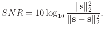
In order to numerically compare the denoising performance, we use the commonly used SNR defined as follows to quantitatively measure the performance (Chen and Fomel, 2015; Gan et al., 2015a; Yang et al., 2015):
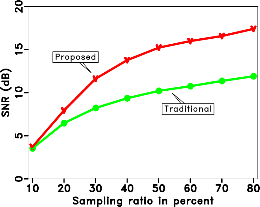
In order to demonstrate the reconstruction performance of the two rank-reduction methods with respect to noise level. We conduct 6 experiments of the 5D data reconstruction based on the first synthetic example, in which we use different noise level in different experiments. We plot the final SNRs using two different approaches after 10 iterations with respect to the noise variances in Figure 11. The red line shows the SNR diagram of the proposed approach and green line shows the SNR diagram of the traditional approach. The noise variance of 6 experiments are 0.05, 0,1, 0.25, 0.5, 0.75, and 1. Please note that all presented examples above are based on the noise variance 0.25. It can be intuitively inferred that noise variance above 0.25 can make the data even noisier. From Figure 11, it is clear that the proposed approach is always superior than the traditional approach in terms of SNR. It is more important to observe that as the noise level increases, the difference in terms of SNR of the two approaches also increases. It offers us a practical guideline that the proposed approach can be best utilized in the condition of strong noise corruption (or in other words on observed data with low SNR), which is usually the feature of most land seismic data. In order to demonstrate the reconstruction performance with respect to sampling ratio of the observed data, we did 8 experiments with different sampling ratios. The SNRs using two approaches after 10 iterations with respect to the sampling ratios are shown in Figure 12. Red line denotes the proposed approach and green line denotes the traditional approach. The proposed approach is always better than the traditional approach and as the sampling ratio increases (in other words we get more and more available traces), the difference between the proposed and traditional approaches increases too.
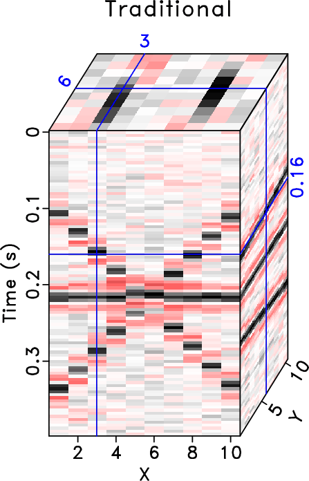
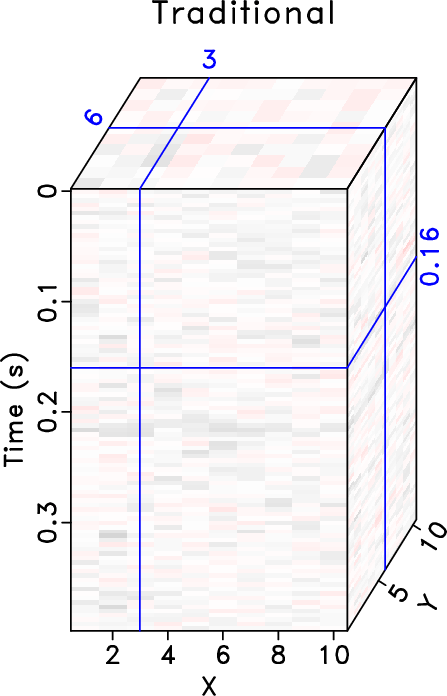
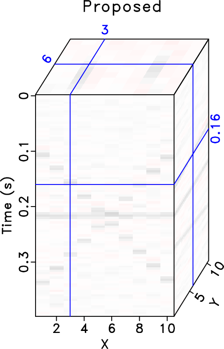
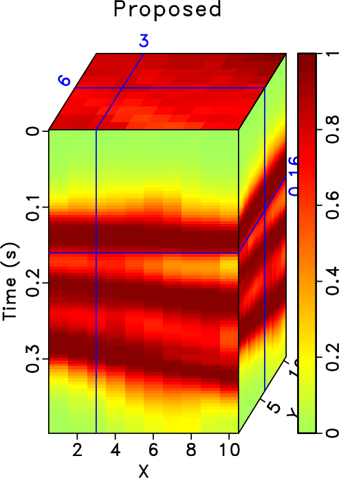
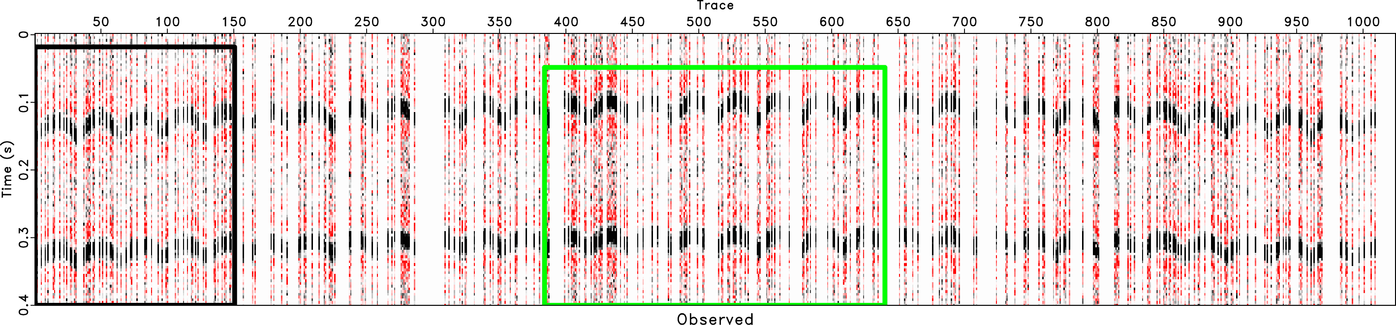
In order to test the effectiveness of the rank-reduction method on data containing curved events and to compare the performances of different methods in this case, we then use the second example to show the performance. In Figure 13, we show a common midpoint gather comparison of the second synthetic example. Here we reshape the 3D data cube into a 2D matrix and compare the performance based on the 2D matrix. Figure 13a shows the clean data. Figure 13b shows the observed data with 70% missing traces and strong random noise. The useful signals are hardly seen from the observed data. After reconstruction using the traditional rank-reduction method with 10 POCS-like iterations, we obtain the reconstructed result as shown in Figure 13c. The result using the proposed approach is shown in Figure 13d. The reconstruction result using the traditional method seems to have significant residual noise and even causes artifacts in some parts of the data. The data highlighted by the green frame boxes are zoomed and shown in Figure 14, where we can have a better view to compare the performance in detail and to see how the proposed method helps recover almost the true model. The data highlighted by the black frame boxes are zoomed and shown in Figure 15, where we can see the artifacts caused by the traditional approach clearly and see the almost perfect performance from the proposed approach. We apply the proposed approach with ![]() and
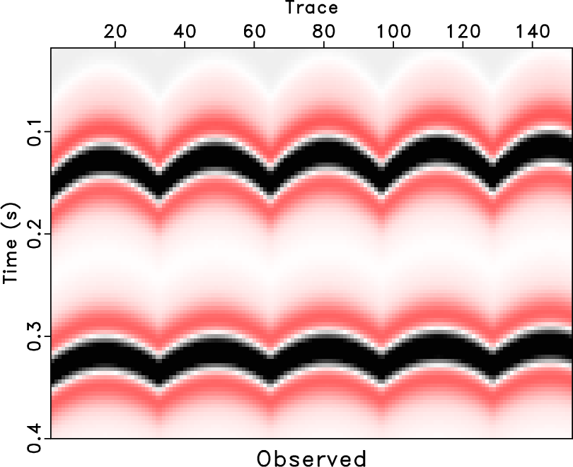
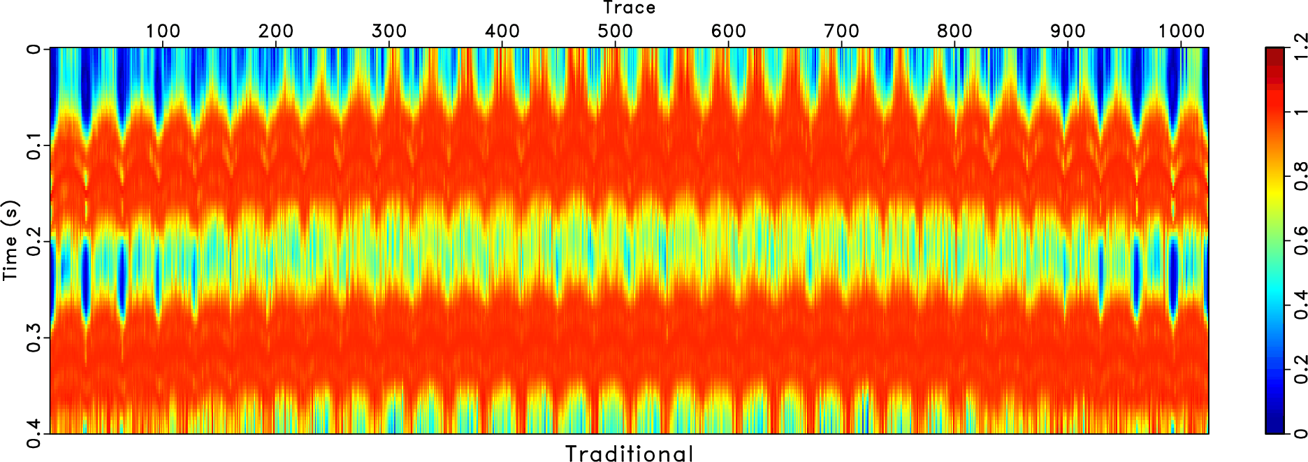
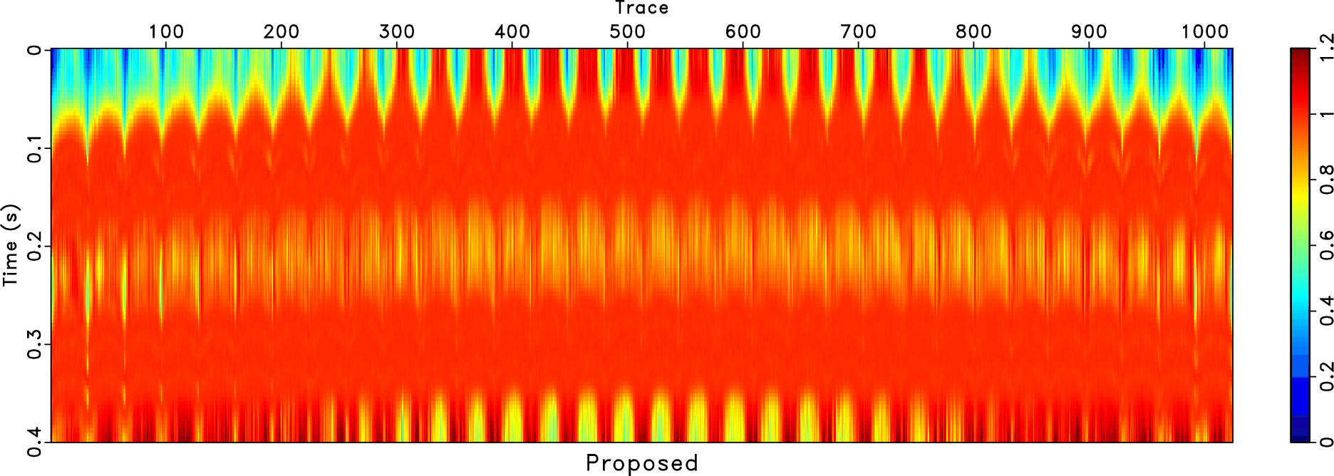
and ![]() for this example. In this dataset, the original SNR of the observed is 0.34 dB. The SNR of the result from traditional rank-reduction approach is 13.56 dB while the SNR of the reconstruction result from the proposed damped rank-reduction method approach is 17.23 dB. In this example, we also calculate the local similarity between different datasets and the clean dataset and show them in Figure 16. Figure 16a shows the local similarity between the observed data and the clean data. Figure 16b shows the local similarity between the result from traditional method and the clean data and Figure 16c shows the local similarity between the result from the proposed method and the clean data. The local similarity vividly demonstrates that the proposed approach can obtain the most similar result to the true model.
for this example. In this dataset, the original SNR of the observed is 0.34 dB. The SNR of the result from traditional rank-reduction approach is 13.56 dB while the SNR of the reconstruction result from the proposed damped rank-reduction method approach is 17.23 dB. In this example, we also calculate the local similarity between different datasets and the clean dataset and show them in Figure 16. Figure 16a shows the local similarity between the observed data and the clean data. Figure 16b shows the local similarity between the result from traditional method and the clean data and Figure 16c shows the local similarity between the result from the proposed method and the clean data. The local similarity vividly demonstrates that the proposed approach can obtain the most similar result to the true model.
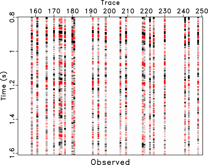
The next example is a field data example. The data has been binned onto a regular grid and a common offset gather of the field data is shown in Figure 17a. Although we are only allowed to show a small portion of the field data and to give a limited discussion based on the performance, the comparison between traditional and proposed rank-reduction methods is adequate to show the superior performance of our proposed method. In the example, about 80% traces are missing from the regular grids. It is obvious that the traditional rank-reduction method obtains a very successful recovery of the missing data, as shown in Figure 17b. However, there are still some residual noise in the reconstructed data, since we use a relatively large ![]() to account for the curved events. We apply the proposed approach with
to account for the curved events. We apply the proposed approach with ![]() and
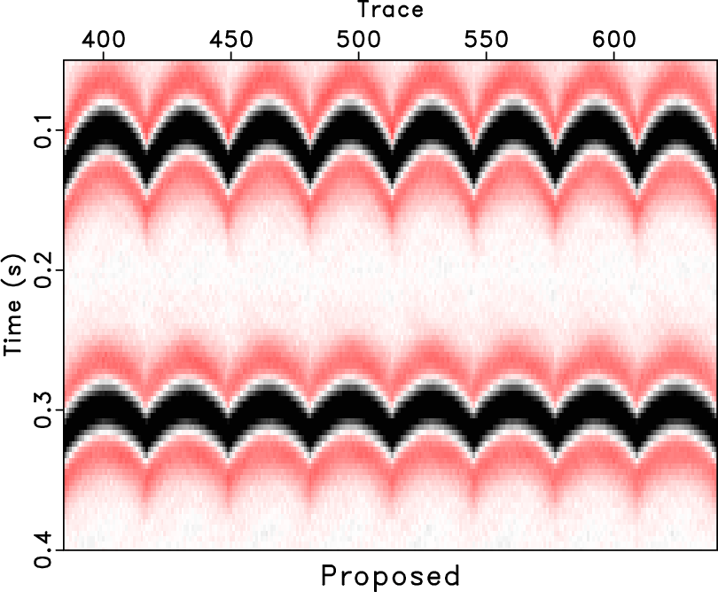
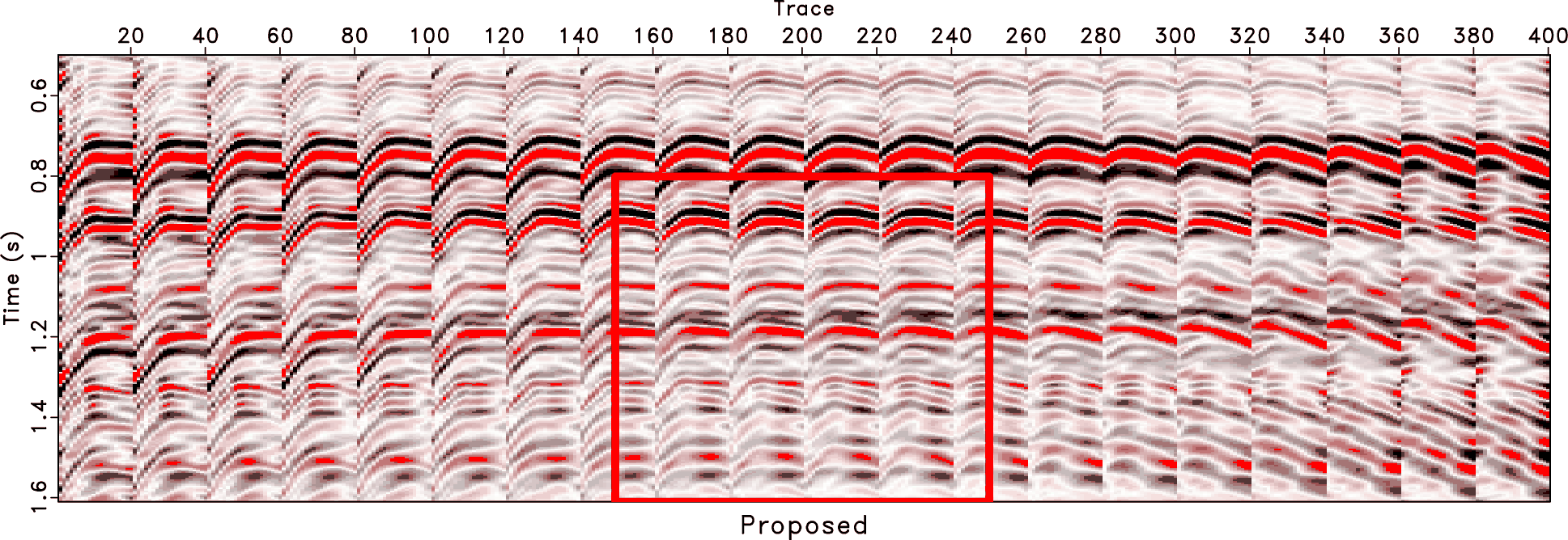
and ![]() and obtain an almost perfect reconstruction performance, as shown in Figure 17c. The events become more coherent and the data becomes much cleaner. We zoom a part from each subfigure in Figure 17 and show the comparison in Figure 18. The zoomed data are highlighted by the red frame boxes shown in Figure 17. The zoomed sections shown in Figure 18 show a clearer comparison between the traditional and the proposed methods, and confirm that the proposed method can obtain a very clean and spatially coherent reconstruction result.
and obtain an almost perfect reconstruction performance, as shown in Figure 17c. The events become more coherent and the data becomes much cleaner. We zoom a part from each subfigure in Figure 17 and show the comparison in Figure 18. The zoomed data are highlighted by the red frame boxes shown in Figure 17. The zoomed sections shown in Figure 18 show a clearer comparison between the traditional and the proposed methods, and confirm that the proposed method can obtain a very clean and spatially coherent reconstruction result.
The selection of rank affects the performance of the traditional rank-reduction based approaches greatly in that smaller value of rank will cause significant damages to the useful signals while larger value of rank will cause serious residual noise left in the reconstructed data. However, it is even impossible to choose an optimal value of rank to stand for the exact signals in practice. In order to preserve as many useful signals as possible, we tend to set a relatively higher value of rank. The proposed approach relieves the dependence of the rank-reduction method on the rank selection since we can use a safe value of rank without compromising the SNR of the final reconstructed data by damping the residual noise that is caused from the increase of rank. In a nutshell, the proposed approach is less sensitive to the value of rank.


|
|---|
|
synth-clean-xy,synth-noisy-xy,synth-obs-xy,synth-rr-xy,synth-drr-xy
Figure 1. Common offset 3D cubes comparison ( |
|
|
|
|---|
|
synth-rr-xy-e,synth-drr-xy-e
Figure 2. Reconstruction error comparison of common offset 3D cubes ( |
|
|


|
|---|
|
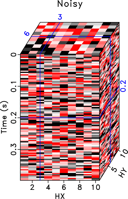
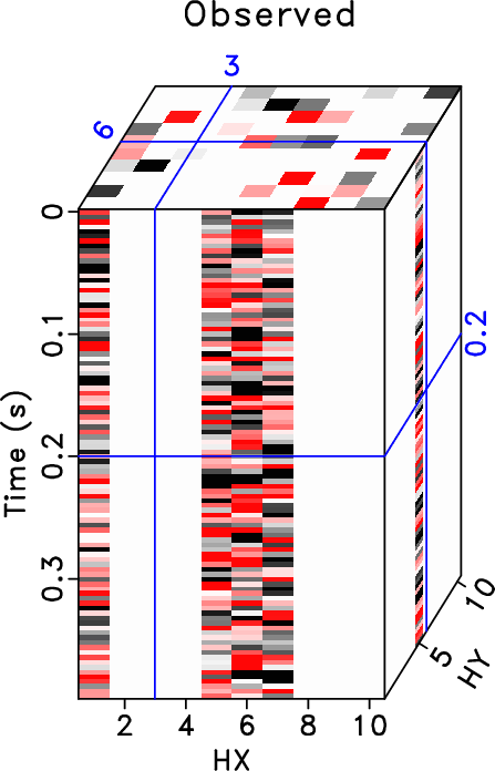
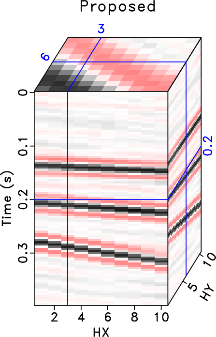
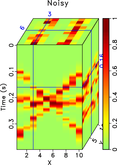
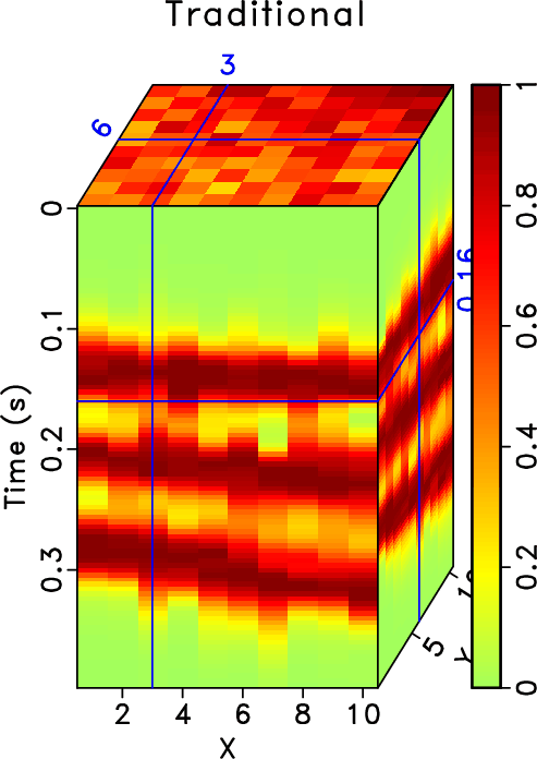
synth-clean-hxhy,synth-noisy-hxhy,synth-obs-hxhy,synth-rr-hxhy,synth-drr-hxhy
Figure 3. Common midpoint 3D cubes comparison ( |
|
|

|
|---|
|
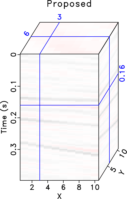
synth-rr-hxhy-e,synth-drr-hxhy-e
Figure 4. Reconstruction error comparison of common midpoint 3D cubes ( |
|
|

|
|---|
|
synth-ss
Figure 5. Comparison of the middle trace amplitude of each cubes in Figure 3. The black line is from the clean data. The red line is from the noisy data. The observed data in this case is zero and thus cannot be seen from the figure.The blue line corresponds to the traditional rank-reduction method. The green line corresponds to the proposed method. Note that the black and green lines are very close to each other, thus the reconstruction error using the proposed approach is much less than the traditional method for most parts. |
|
|

|
|---|
|
H_clean-0,H_obs-0,H_rr10-0,H_drr10-0
Figure 6. 26 Hz block Hankel matrix comparison. (a) Hankel matrix of the clean data. (b) Hankel matrix of the noisy data. (c) Hankel matrix of traditional method after 10 iterations. (d) Hankel matrix of the proposed method after 10 iterations. Please note the erratic artifacts shown in (c), which cannot be handled using the traditional rank-reduction method. The Hankel matrix of the proposed approach is, however, much closer to the true Hankel matrix. |
|
|


|
|---|
|
H-z-clean,H-z-obs,H-z-rr10,H-z-drr10
Figure 7. A close up look of the Hankel matrix (corresponding to the block Hankel matrix highlighted by the green frame box in Figure 6. (a) Hankel matrix of the clean data. (b) Hankel matrix of the noisy data. (c) Hankel matrix of traditional method after 10 iterations. (d) Hankel matrix of the proposed method after 10 iterations. |
|
|


|
|---|
|
H_rr1-0,H_drr1-0,H-z-rr1,H-z-drr1
Figure 8. 26 Hz block Hankel matrix comparison after 1 iteration between two approaches. (a) Hankel matrix of traditional method after 1 iteration. (b) Hankel matrix of the proposed method after 1 iteration. (c)&(d) A close up look of the two frame boxes in (a) and (b). |
|
|


|
|---|
|
synth-noisy-xy-simi,synth-obs-xy-simi,synth-rr-xy-simi,synth-drr-xy-simi
Figure 9. Local similarity comparison of common offset 3D cubes comparison ( |
|
|


|
|---|
|
synth-noisy-hxhy-simi,synth-obs-hxhy-simi,synth-rr-hxhy-simi,synth-drr-hxhy-simi
Figure 10. Local similarity comparison of common midpoint 3D cubes ( |
|
|

|
|---|
|
snr-n
Figure 11. SNR diagrams of the different approaches with respect to the noise level (variance value). Note that the proposed approach outperforms the traditional methods more and more as the noise level increases. |
|
|
|
|---|
|
snr-r
Figure 12. SNR diagrams of the different approaches with respect to the sampling ratio (in percent). |
|
|


|
|---|
|
hyper-clean2d-1,hyper-obs2d-1,hyper-rr2d-1,hyper-drr2d-1
Figure 13. Common midpoint gather comparison (reshaped into a 2D matrix). (a) Clean synthetic data with curved events. (b) Observed synthetic data (with 70% missing traces and strong noise). (c) Reconstructed data using the traditional approach. (d) Reconstructed data using the proposed approach. |
|
|


|
|---|
|
hyper-z-clean,hyper-z-obs,hyper-z-rr,hyper-z-drr
Figure 14. Zoomed sections from Figure 13 (the green frame box). (a) Clean data. (b) Observed data. (b) Reconstructed data using the traditional approach. (c) Reconstructed data using the proposed approach. |
|
|


|
|---|
|
hyper-z1-clean,hyper-z1-obs,hyper-z1-rr,hyper-z1-drr
Figure 15. Zoomed sections from Figure 13 (the black frame box). (a) Clean data. (b) Observed data. (b) Reconstructed data using the traditional approach. (c) Reconstructed data using the proposed approach. Note the strong artifacts caused from the traditional approach. |
|
|

|
|---|
|
hyper-obs-simi,hyper-rr-simi,hyper-drr-simi
Figure 16. Local similarity comparison with respect to the clean data. (a) Similarity of the Observed synthetic data. (b) Similarity of the reconstructed data using the traditional approach. (c) Similarity of the reconstructed data using the proposed approach. |
|
|


|
|---|
|
field-obs2d-0,field-rr2d0-0,field-drr2d-0
Figure 17. Common offset gather comparison (reshaped into a 2D matrix). (a) Observed field data (with 80% missing traces). (b) Reconstructed data using the traditional approach. (c) Reconstructed data using the proposed approach. |
|
|


|
|---|
|
z-obs,z-rr,z-drr
Figure 18. Zoomed sections from Fig 17. (a) Observed field data. (b) Reconstructed data using the traditional approach. (c) Reconstructed data using the proposed approach. |
|
|
|
|
|
|
Simultaneous denoising and reconstruction of 5D seismic data via damped rank-reduction method |