 |
 |
 |
 | Elastic wave-vector decomposition in heterogeneous anisotropic media |  |
![[pdf]](icons/pdf.png) |
Next: Low-rank approximations for wave-vector
Up: Review of wave-mode separation
Previous: Elastic wave-mode separation
Wave-vector decomposition aims to decompose wavefields in the wavenumber domain via a projection operator. For homogeneous isotropic media,
Zhang and McMechan (2010) proposed to rewrite equations 1 and 2 as
 and and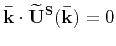 |
(6) |
and
 and and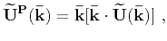 |
(7) |
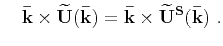
As follows from equations 6 and 7, the following equivalent expressions are (Zhang and McMechan, 2010)
![$\displaystyle \mathbf{\widetilde{U}^P(\bar{k})} = \mathbf{\bar{k}}[\mathbf{\bar{k}}\cdot\mathbf{\widetilde{U}(\bar{k})}]~,$](img55.png) |
(8) |
and
![$\displaystyle \mathbf{\widetilde{U}^S(\bar{k})} = -\mathbf{\bar{k}}\times[\mathbf{\bar{k}}\times\mathbf{\widetilde{U}(\bar{k})}]~.$](img56.png) |
(9) |
The expressions corresponding to equations 8 and 9 in homogeneous TI media are
![$\displaystyle \mathbf{\widetilde{U}^{P}(\bar{k})} = \mathbf{a^{P}(\bar{k})}[\mathbf{a^{P}(\bar{k})}\cdot\mathbf{\widetilde{U}(\bar{k})}]$](img57.png) |
(10) |
and
![$\displaystyle \mathbf{\widetilde{U}^{S}(\bar{k})} = -\mathbf{a^{P}(\bar{k})}\times[\mathbf{a^{P}(\bar{k})}\times\mathbf{\widetilde{U}(\bar{k})}]~,$](img58.png) |
(11) |
where
 contains the wavefield corresponding to both S-wave modes.
Equation 10 was originally proposed by Dellinger (1991). To decompose a vector wavefield, one can use either equation 10 or equation 11 and polarization vectors obtained from solving the Christoffel equation. Following equation 10, we can decompose the wavefield in a homogeneous TI medium as follows:
contains the wavefield corresponding to both S-wave modes.
Equation 10 was originally proposed by Dellinger (1991). To decompose a vector wavefield, one can use either equation 10 or equation 11 and polarization vectors obtained from solving the Christoffel equation. Following equation 10, we can decompose the wavefield in a homogeneous TI medium as follows:
Following equation 11, we can decompose the wavefield in a homogeneous TI medium as follows:
The handling of heterogeneity can be done in a similar fashion to the wave-mode separation case where the polarizations become functions of both spatial location and normalized wave-vector. Because the wave-vector decomposition defined in equations 12 and 13 satisfies the linear superposition relation, the three separated wavefields are orthogonal to one another, while their amplitude, phase, and other physical properties are correctly preserved, unlike the results from the wave-mode separation in equations 4 and 5.
To extend the wave-vector decomposition to low-symmetry anisotropic media, we follow the scheme in equation 12 and utitlize the projection operator for the 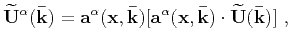 wave mode given by
![$\displaystyle \mathbf{\widetilde{U}^{\alpha}}(\mathbf{\bar{k}}) = \mathbf{a}^{\...
...a}^{\alpha}(\mathbf{x},\mathbf{\bar{k}})\cdot\mathbf{\widetilde{U}(\bar{k})}]~,$](img72.png) |
(14) |
where the heterogeneity is taken into account via the dependence of the polarization vector
 on spatial location
 and normalized wave-vector
 . We discuss the suitable definitions of wave modes in low-symmetry anisotropic media in a later section.
|
|
|
|
| Elastic wave-vector decomposition in heterogeneous anisotropic media | |
|
Next: Low-rank approximations for wave-vector
Up: Review of wave-mode separation
Previous: Elastic wave-mode separation
2017-04-18