|
|
|
|
Elastic wave-vector decomposition in heterogeneous anisotropic media |
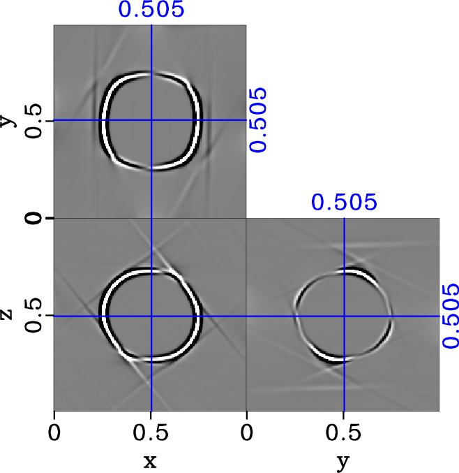
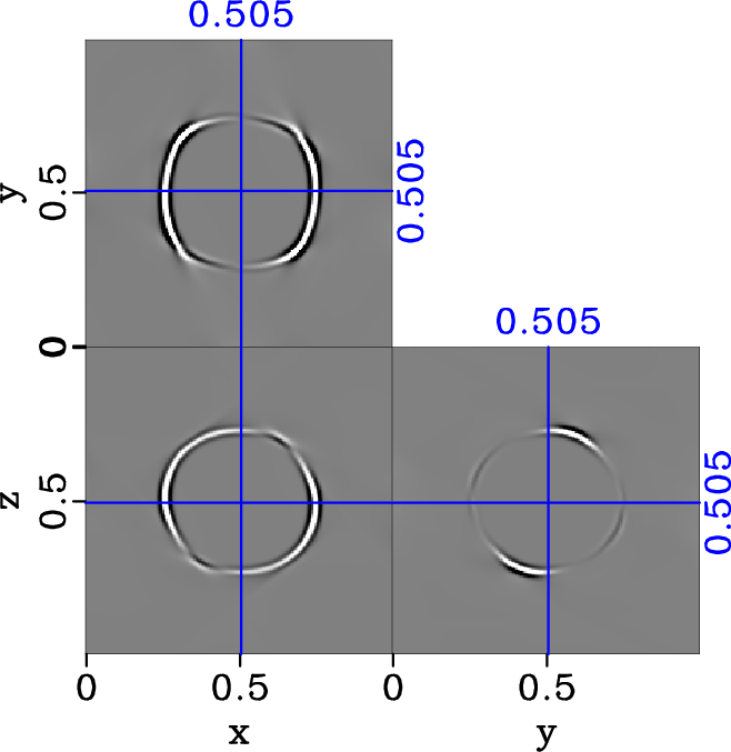
 . We observe a complicated behavior of the two S-wave modes in comparison with the orthorhombic case in Figure 7. We show only the y-component of the separated S1 and S2 wavefields in Figures 12 and 13 for conciseness. We observe reduced planar artifacts after the implementation of the proposed smoothing method and further correct the amplitudes. The y-component of the resultant separated wavefields with and without corrected amplitudes are shown in comparison in Figure 12. We observe again clean separated wavefields with no apparent artifacts and correct amplitudes similar to the previous case of homogeneous orthorhombic model.


|
|---|
|
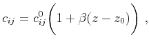
hTRIw-lr-x,hTRIw-lr-y,hTRIw-lr-z
Figure 11. Original elastic wavefield in |
|
|

|
|---|
|
nohTRIw-dlr-S1-y,hTRIw-dlr-S1-y,comhTRIw-dlr-S1-y
Figure 12. Separated y-component of S1 elastic wavefield in the triclinic model (equation 20) with |
|
|


|
|---|
|
nohTRIw-dlr-S2-y,hTRIw-dlr-S2-y,comhTRIw-dlr-S2-y
Figure 13. Separated y-component of S2 elastic wavefield in the triclinic model (equation 20) with |
|
|
|
|
|
|
Elastic wave-vector decomposition in heterogeneous anisotropic media |