|
|
|
|
Fractal heterogeneities in sonic logs and low-frequency scattering attenuation |
We propose to use the synthesis of a random medium
detailed in Table 2 for ![]() =1
as a basis for the procedure to estimate heterogeneity parameters from sonic logs.
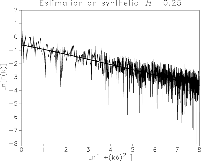
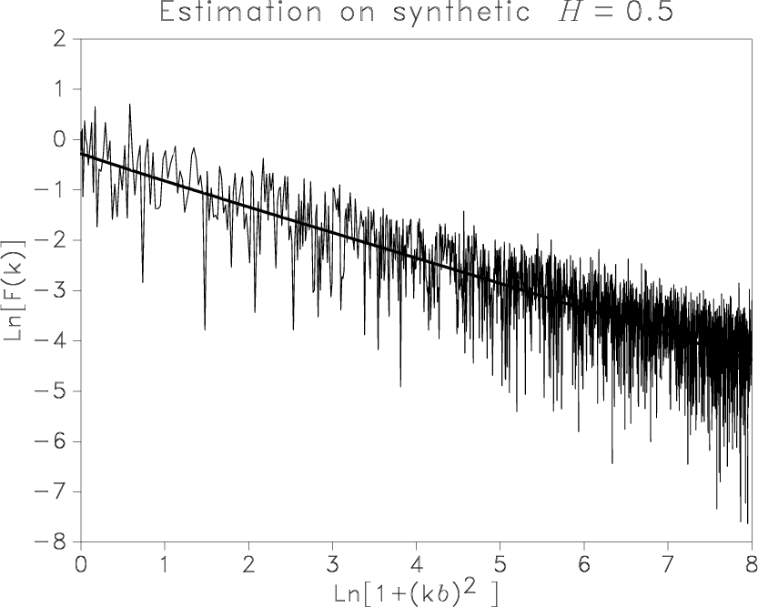
We achieve optimization by using a weighted least-squares method in the spectral domain
on the logarithm of the amplitude, with the model derived from equation 7:
=1
as a basis for the procedure to estimate heterogeneity parameters from sonic logs.
We achieve optimization by using a weighted least-squares method in the spectral domain
on the logarithm of the amplitude, with the model derived from equation 7:
|
|---|
|
cgaussM025,lligaussfM025,cgauss025,lligaussf025,cgauss05,lligaussf05
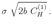
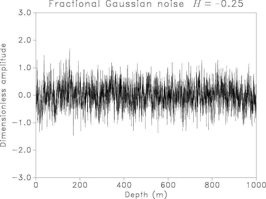
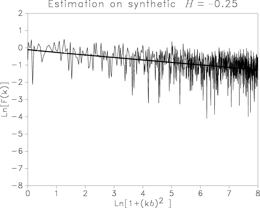
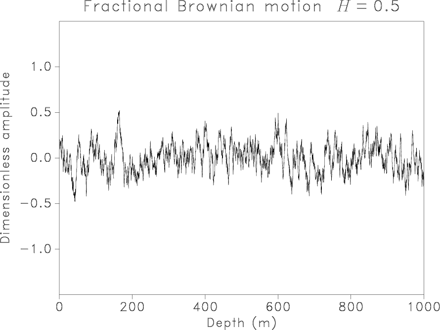
Figure 2. Synthetic signals generated as fGn with |
|
|
|
|---|
|
signalA1,signalC2,llisignalfA1,llisignalfC2,rllisignalfA1L,rllisignalfC2L
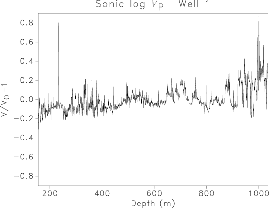
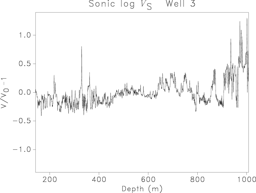
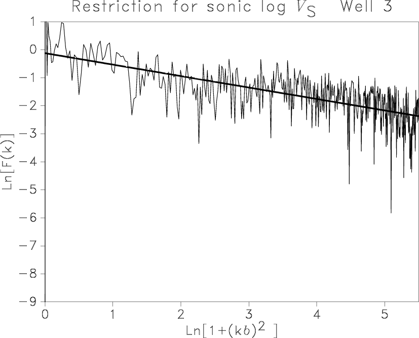
Figure 3. Sonic log |
|
|
| Parameters | |||
| Generated fGn | -0.25 | 10.0 | 20 |
| Recovered | -0.21 | 11.0 | 18 |
| Generated fGn | -0.25 | 5.0 | 20 |
| Recovered | -0.21 | 5.9 | 17 |
| Generated fBm | 0.25 | 10.0 | 30 |
| Recovered | 0.26 | 10.2 | 23 |
| Generated fBm | 0.50 | 5.0 | 40 |
| Recovered | 0.51 | 5.3 | 32 |
| Generated fBm | 0.75 | 3.0 | 40 |
| Recovered | 0.79 | 2.7 | 30 |
Well log data come from a sandy channel reservoir with a clastic overburden,
and the facies evolves from silty sandstone to mudstone,
which is characteristic of alluvial deposition.
Velocities ![]() and
and ![]() were both measured with a spatial sampling of
were both measured with a spatial sampling of ![]() m.
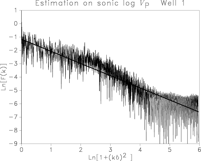
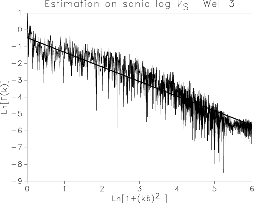
Figure 3 shows
the parameter estimation for two sonic logs.
Comparison with the method applied to the synthetics in
Figure 2
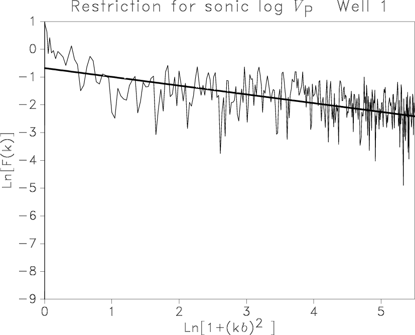
uncovers the existence of different slopes for different frequencies in Figures 3c and 3d.
We can reasonably delimit three domains, denoted (A) for low frequencies, (B) for medium frequencies, and (C) for very high frequencies.
These domains can be identified by parameters
m.
Figure 3 shows
the parameter estimation for two sonic logs.
Comparison with the method applied to the synthetics in
Figure 2
uncovers the existence of different slopes for different frequencies in Figures 3c and 3d.
We can reasonably delimit three domains, denoted (A) for low frequencies, (B) for medium frequencies, and (C) for very high frequencies.
These domains can be identified by parameters ![]() and
and ![]() , representing specific values of relative distance
, representing specific values of relative distance ![]() , namely
, namely
Results are summarized in Table 4
for the four different sonic logs ![]() and
and ![]() .
The ratio
.
The ratio
![]() is almost constant
for the four well logs and roughly equal to two.
The updated estimation in the spatial wavelength domain (A) produces reasonable results in Table 4.
Standard deviation
is almost constant
for the four well logs and roughly equal to two.
The updated estimation in the spatial wavelength domain (A) produces reasonable results in Table 4.
Standard deviation ![]() varies from 20 to 45 %
and is larger for
varies from 20 to 45 %
and is larger for ![]() logs than for
logs than for ![]() logs.
Correlation length
logs.
Correlation length ![]() is about 5 m for both
is about 5 m for both ![]() and
and ![]() ,
except for the well N
,
except for the well N![]() 4, which is 2.5 m.
Exponent
4, which is 2.5 m.
Exponent ![]() for
for ![]() varies from 0.1 to 0.4
and for
varies from 0.1 to 0.4
and for ![]() from 0.2 to 0.6.
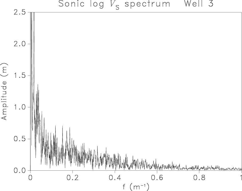
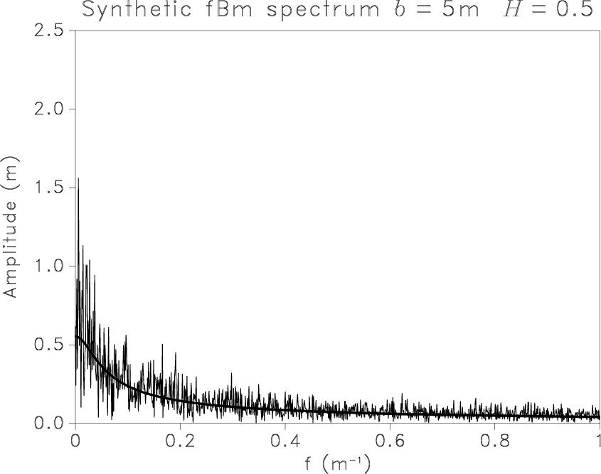
In Figure 4,
comparison of the frequency content of one real sonic log
with one realization of a synthetic fBm, generated using similar parameters, shows that
the sonic-log data contain higher peaks for very large wavelengths.
We detected in the different sonic well logs the recurrence of some particular spatial cycles
at 2.5 m, 5 m, 10 m, and 20 m.
from 0.2 to 0.6.
In Figure 4,
comparison of the frequency content of one real sonic log
with one realization of a synthetic fBm, generated using similar parameters, shows that
the sonic-log data contain higher peaks for very large wavelengths.
We detected in the different sonic well logs the recurrence of some particular spatial cycles
at 2.5 m, 5 m, 10 m, and 20 m.
| Well Log | b (m) |
|
||
| N |
0.79 | 1.32 | 17 | 2791 |
| 6.70 | 0.13 | 22 | ||
| 1.05 | 1.16 | 32 | 1218 | |
| 5.92 | 0.21 | 35 | ||
| N |
1.90 | 0.92 | 27 | 2842 |
| 5.34 | 0.38 | 29 | ||
| 2.84 | 0.83 | 45 | 1240 | |
| 3.08 | 0.62 | 44 | ||
| N |
1.34 | 1.16 | 20 | 2787 |
| 7.22 | 0.18 | 21 | ||
| 1.25 | 1.23 | 32 | 1216 | |
| 5.01 | 0.32 | 36 | ||
| N |
0.64 | 1.98 | 18 | 2745 |
| 2.58 | 0.39 | 38 | ||
| 0.57 | 2.26 | 32 | 1247 | |
| 2.46 | 0.56 | 33 |
|
|---|
|
rfsignalC2,fitfiltb025
Figure 4. Fourier spectrum of the scaled |
|
|
|
|
|
|
Fractal heterogeneities in sonic logs and low-frequency scattering attenuation |