|
|
|
|
Fractal heterogeneities in sonic logs and low-frequency scattering attenuation |
| Steps | Domain | Operation for fGn | Operation for fBm |
| 1 | Space | Generate Gaussian white noise |
|
| 2 | Fourier | Generate energy spectrum
|
|
| 3 | Fourier |
 |
 |
| 4 | Space | Obtain correlated fGn |
Obtain correlated fBm |
Our method of synthesizing correlated random media is summarized in Table 2
for fractional Gaussian noise (fGn) and fractional Brownian motion (fBm).
The Gaussian nature of the initial white noise is contained in the phase of its Fourier transform ![]() ,
whereas the amplitude is constant with frequency because the noise is white.
The causal integration, to produce the fBm, is performed by a phase rotation in the Fourier domain, strictly equivalent to the Hilbert transform.
The fractal property, below spatial scale
,
whereas the amplitude is constant with frequency because the noise is white.
The causal integration, to produce the fBm, is performed by a phase rotation in the Fourier domain, strictly equivalent to the Hilbert transform.
The fractal property, below spatial scale ![]() , is imposed by the amplitude
, is imposed by the amplitude
 of the von Kármán model.

|
|---|
|
signal,f2dfile,cgaussb,fcgaussbp
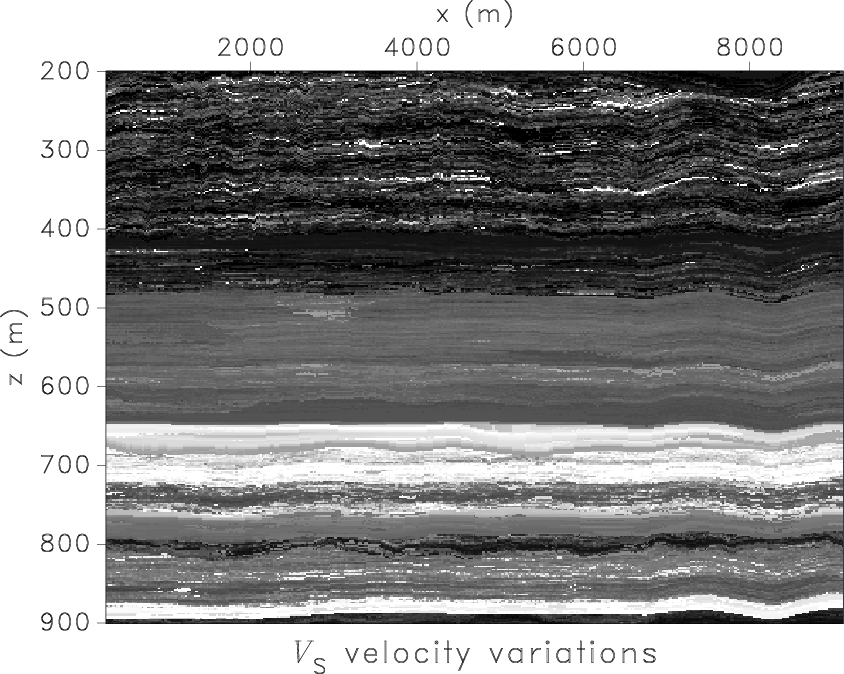
Figure 1. Variations of |
|
|
For dimension ![]() , the exponent in equation 7 is
, the exponent in equation 7 is ![]() .
Therefore, the energy spectrum of the 2D fGn with
.
Therefore, the energy spectrum of the 2D fGn with ![]() in Figure 1
is
in Figure 1
is
![]() .
Klimes (2002) in fact proposed using
.
Klimes (2002) in fact proposed using
![]() to synthesize geologically realistic 2D models
with the von Kármán function.
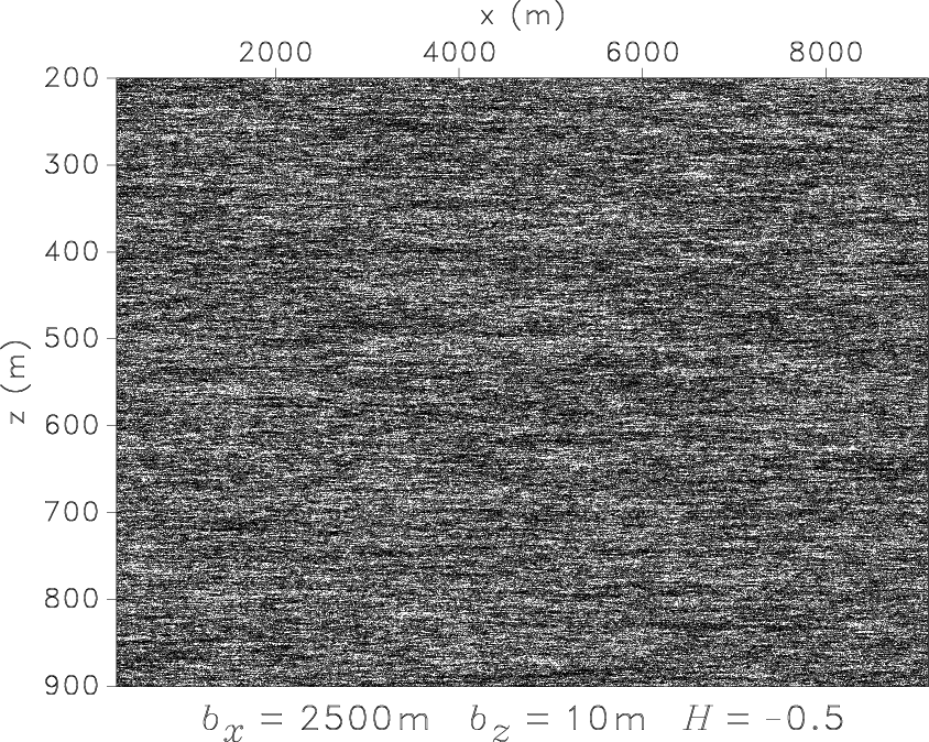
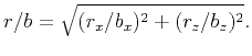
Because sediments are made up of layers, we consider the autocorrelation function to be vertical transverse isotropic.
We use two different correlation lengths
to synthesize geologically realistic 2D models
with the von Kármán function.
Because sediments are made up of layers, we consider the autocorrelation function to be vertical transverse isotropic.
We use two different correlation lengths ![]() and
and ![]() for horizontal and vertical directions,
and define the Riemannian relative distance (Goff and Jordan, 1988):
for horizontal and vertical directions,
and define the Riemannian relative distance (Goff and Jordan, 1988):
 |
(12) |
|
|
|
|
Fractal heterogeneities in sonic logs and low-frequency scattering attenuation |