Traveltime approximations for transversely isotropic media with an inhomogeneous background

Appendix B: Expansion in $\theta$ and $\eta$

For an expansion in $\theta$ and $\eta$, simultaneously, I use the following trial solution:

$$\tau(x,z) \approx \tau_{0}(x,z) +\tau_{\eta}(x,z) \eta+\tau... ...ta}(x,z) \eta \sin\theta+ \tau_{\theta_2}(x,z) \sin^{2}\theta,$$ (30)

in terms of the coefficients $\tau_{i}$, where the $i$ corresponds to $\eta,\theta,\eta_2,\eta \theta$, and $\theta_2$. Inserting the trial solution, equation B-1, into equation A-1 yields again a long formula, but by setting both $\sin\theta=0$ and $\eta=0$, I obtain the zeroth-order term given by

$$v^2(x,y,z) \left(\frac{\partial \tau_{0}}{\partial x}\right)... ...,z) \left(\frac{\partial \tau_{0}}{\partial z}\right)^2 = 1\;,$$ (31)

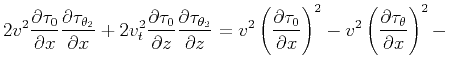
which is simply the eikonal formula for elliptical anisotropy. By equating the coefficients of the powers of the independent parameter $\sin\theta$ and $\eta$, in succession starting with first powers of the two parameters, we end up first with the coefficients of first-power in $\sin\theta$ and zeroth power in $\eta$, simplified by using equation B-2, and given by

$$v^2 \frac{\partial \tau_{0}}{\partial x} \frac{\partial \ta... ...l \tau_{0}}{\partial x} \frac{\partial \tau_{0}}{\partial z},$$ (32)

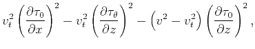
which is a first-order linear partial differential equation in $\tau_{\theta}$. The coefficients of zero-power in $\sin\theta$ and the first-power in $\eta$ is given by

$$v^2 \frac{\partial \tau_{0}}{\partial x} \frac{\partial \ta... ...2 \left(\frac{\partial \tau_{0}}{\partial z}\right)^2\right),$$ (33)

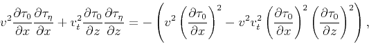
The coefficients of the square terms in $\sin\theta$, with some manipulation, results in the following relation

$$2 v^2 \frac{\partial \tau _{0}}{\partial x} \frac{\partial \tau ... ...al x}\right)^2-v^2 \left(\frac{\partial \tau _{\theta}}{\partial x}\right)^2-$$

$$2 \left(v^{2}-v_t^{2}\right) \frac{\partial \tau _{\theta}}{\par... ...ac{\partial \tau _{0}}{\partial x} \frac{\partial \tau _{\theta}}{\partial z}-$$

$$v_t^2 \left(\frac{\partial \tau _{0}}{\partial x}\right)^2-v_t^2... ...ft(v^{2}-v_t^{2}\right) \left(\frac{\partial \tau _{0}}{\partial z}\right)^2,$$ (34)

which is again a first-order linear partial differential equation in $\tau_{\theta_2}$ with an obviously more complicated source function given by the right hand side. The coefficients of the square terms in $\eta$, with also some manipulation, results in the following relation

$$2 v^2 \frac{\partial \tau _{0}}{\partial x} \frac{\partial \tau ... ...artial \tau _{0}}{\partial x} \frac{\partial \tau _{\eta}}{\partial z}\right)-$$

$$v^2 \left(\frac{\partial \tau _{\eta}}{\partial x}\right)^2- 4 v... ...}}{\partial x}-v_t^2 \left(\frac{\partial \tau _{\eta}}{\partial z}\right)^2,$$ (35)

which is again a first-order linear partial differential equation in $\tau_{\eta_2}$ with a again complicated source function.

Finally, the coefficients of the first-power terms in both $\sin\theta$ and $\eta$ results also in a first-order linear partial differential equation in $\tau_{\eta \theta}$ given by

$$2 v^2 \frac{\partial \tau _{0}}{\partial x} \frac{\partial \tau ... ...rtial \tau _{0}}{\partial z} \frac{\partial \tau _{\eta \theta}}{\partial z} =$$

$$4 v_t^2 v^2 \frac{\partial \tau _{0}}{\partial x} \frac{\partial ... ...tau _{\theta}}{\partial z}-\frac{\partial \tau _{0}}{\partial x}\right)\right)$$

$$-2 v^2 \frac{\partial \tau _{0}}{\partial x} \frac{\partial \tau... ...rtial \tau _{\theta}}{\partial x}+\frac{\partial \tau _{0}}{\partial z}\right)$$

$$+2 v_t^2 \frac{\partial \tau _{\eta}}{\partial x} \frac{\partial... ...tial \tau _{\theta}}{\partial z}-\frac{\partial \tau _{0}}{\partial x}\right).$$ (36)

Though the equation seems complicated, many of the variables of the source function (right hand side) can be evaluated during the evaluation of equations B-3 and B-4 in a fashion that will not add much to the cost.

Using Shanks transforms (Bender and Orszag, 1978) we can isolate and remove the most transient behavior of the expansion B-1 in $\eta$ (the $\theta$ expansion did not improve with such a treatment) by first defining the following parameters:

$$A_0 = \tau_{0}+ \tau_{\theta} \sin\theta+ \tau_{\theta_2} \sin^{2}\theta$$

$$A_1 = A_{0} + \left(\tau_{\eta}+ \tau_{\eta \theta} \sin\theta \right) \eta$$

$$A_2 = A_{1} + \tau_{\eta_2} \eta^2$$ (37)

The first sequence of Shanks transforms uses $A_0$, $A_1$, and $A_2$, and thus, is given by

$$\tau(x,z) \approx \frac{A_0 A_2-A_1^2}{A_0-2 A_1+A_2} = \tau_{0}(x,z)+ \tau_{\theta}(x,z) \sin\theta+ \tau_{\theta_2}(x,z) \sin^{2}\theta$$

$$+\frac{\eta \left(\tau_{\eta}(x,z)+ \tau_{\eta \theta}(x,z) \sin\... ...tau_{\eta}(x,z)+ \tau_{\eta \theta}(x,z) \sin\theta -\eta \tau _{\eta_2}(x,z)}.$$ (38)

Traveltime approximations for transversely isotropic media with an inhomogeneous background