 |
 |
 |
 | Time migration velocity analysis by velocity continuation |  |
![[pdf]](icons/pdf.png) |
Next: Finite-difference approach
Up: Fomel: Velocity continuation
Previous: Introduction
The post-stack velocity continuation process is governed by a partial
differential equation in the domain, composed by the seismic image
coordinates (midpoint  and vertical time
  ) and the additional
velocity coordinate
) and the additional
velocity coordinate  . Neglecting some amplitude-correcting terms
(Fomel, 2003), the equation takes the form
(Claerbout, 1986)
. Neglecting some amplitude-correcting terms
(Fomel, 2003), the equation takes the form
(Claerbout, 1986)
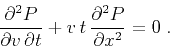 |
(1) |
Equation (1) is linear and belongs to the hyperbolic type. It
describes a wave-type process with the velocity acting as a
propagation variable. Each constant- slice of the function
 corresponds to an image with the corresponding constant
velocity. The necessary boundary and initial conditions are
corresponds to an image with the corresponding constant
velocity. The necessary boundary and initial conditions are
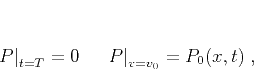 |
(2) |
where  is the starting velocity,
  for continuation to a smaller
velocity and
for continuation to a smaller
velocity and  is the largest time on the image (completely attenuated
reflection energy) for continuation to a larger velocity. The first case
corresponds to ``modeling'' (demigration); the latter case, to seismic
migration.
is the largest time on the image (completely attenuated
reflection energy) for continuation to a larger velocity. The first case
corresponds to ``modeling'' (demigration); the latter case, to seismic
migration.
Mathematically, equations (1) and (2) define a
Goursat-type problem (Courant and Hilbert, 1989). Its analytical solution can be
constructed by a variation of the Riemann method in the form of an
integral operator (Fomel, 2003,1994):
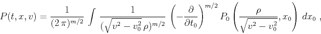 |
(3) |
where
 ,
,  in the 2-D
case, and
in the 2-D
case, and  in the 3-D case. In the case of continuation from zero
velocity
in the 3-D case. In the case of continuation from zero
velocity  , operator (3) is equivalent (up to the
amplitude weighting) to conventional Kirchoff time migration
(Schneider, 1978). Similarly, in the frequency-wavenumber
domain, velocity continuation takes the form
, operator (3) is equivalent (up to the
amplitude weighting) to conventional Kirchoff time migration
(Schneider, 1978). Similarly, in the frequency-wavenumber
domain, velocity continuation takes the form
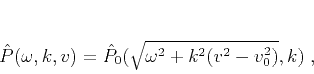 |
(4) |
which is equivalent (up to scaling coefficients) to Stolt migration
(Stolt, 1978), regarded as the most efficient constant-velocity
migration method.
If our task is to create many constant-velocity slices, there are
other ways to construct the solution of problem (1-2).
Two alternative approaches are discussed in the next two
subsections.
Subsections
|
|
|
|
| Time migration velocity analysis by velocity continuation | |
|
Next: Finite-difference approach
Up: Fomel: Velocity continuation
Previous: Introduction
2013-03-03