next up previous [pdf]

Next: Conclusions Up: Fomel & Biondi: t-x Previous: CASCADING DMO AND INVERSE

AMO APERTURE: CASCADING MIGRATION AND MODELING

The impulse response of the AMO operators corresponds to a spike on the initial constant-offset constant-azimuth gather. Such a spike can physically occur in the case of a focusing ellipsoidal reflector whose focuses are coincident with the initial source and receiver locations (the impulse response of prestack common-offset migration). Therefore, the impulse response of AMO corresponds kinematically to a reflection from this ellipsoid. These considerations allow us to define AMO as the cascade of the 3-D common-offset common-azimuth migration and the 3-D modeling for a different azimuth and offset. An analogous point of view was developed for the 2-D case by Deregowski and Rocca (1981).

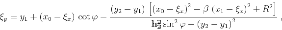
Let's consider the general symmetric ellipsoid equation

\begin{displaymath}
z(x,y)=\sqrt{R^2-\beta \left(x-x_1\right)^2-\left(y-y_1\right)^2}\;,
\end{displaymath} (15)

where $z$ stands for the depth coordinate, $R$ is the small semi-axis of the ellipsoid, and $\beta$ is a nondimensional parameter describing the stretching of the ellipse $(\beta < 1)$. Deregowski and Rocca (1981) derived the following connections between the geometric properties of the reflector and the coordinates of the corresponding spike in the data:
\begin{displaymath}
R={{v t_1}\over 2}\;;\;
\beta={t_1^2 \over t_1^2+{{4 {\bf h_1}^2}\over v^2}}\;,
\end{displaymath} (16)

where $v$ is the wave velocity. The center of the ellipsoid is at the initial midpoint ${\bf x_1}$.

This section addresses the kinematic problem of reflection from the ellipsoid defined by (15). In particular, we are looking for the answer to the following question: For a given elliptic reflector defined by the input midpoint, offset, and time coordinates, what points on the surface can form a source-receiver pair valid for a reflection? If a point in the output midpoint-offset space cannot be related to a reflection pattern, we should exclude it from the AMO impulse response defined in (1).

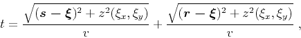
Fermat's principle provides a general method of solving the kinematic reflection problems. Consider a formal expression for the two-point reflection traveltime

\begin{displaymath}
t={\sqrt{
(\mbox{\boldmath {$s - \xi$}})^2+z^2(\xi_x,\xi_y)}...
...(\mbox{\boldmath {$r - \xi$}})^2+z^2(\xi_x,\xi_y)}
\over v}\;,
\end{displaymath} (17)

where $\xi=$ $\left\{\xi_x,\xi_y\right\}$ is the vertical projection of the reflection point to the surface, ${\bf s}=\left\{s_x,s_y\right\}={\bf x_2-h_2}$ is the source location, and ${\bf r}=\left\{r_x,r_y\right\}={\bf x_2+h_2}$ is the receiver location. According to Fermat's principle, the reflection ray path between two fixed points must correspond to the extremum value of the traveltime. Hence, in the vicinity of a reflected ray,
\begin{displaymath}
{\partial t \over \partial \xi_x}=0\;;\;
{\partial t \over \partial \xi_y}=0\;.
\end{displaymath} (18)

Solving the system of equations (18) for $\xi_x$ and $\xi_y$ allows us to find the reflection ray path for a given source-receiver pair on the surface. The solution is derived in Appendix B to be
\begin{displaymath}
\xi_x={{x_0-\beta x_1}\over{1-\beta}}\;,
\end{displaymath} (19)


\begin{displaymath}
\xi_y=y_1+\left(x_0-\xi_x\right) \cot{\varphi}-
{{\left(y_2...
...}\over
{{\bf h_2^2}\sin^2{\varphi}-\left(y_2-y_1\right)^2}}\;,
\end{displaymath} (20)

where $x_0$ has the same meaning as in the preceding section and is defined by (7).

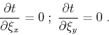
Since the reflection point is contained inside the ellipsoid, its projection obeys the evident inequality

\begin{displaymath}
\left(\xi_y-y_1\right)^2\leq R^2-\beta \left(\xi_x-x_1\right)^2\;.
\end{displaymath} (21)

It is inequality (21) that defines the aperture of the AMO operator.

amoapp
amoapp
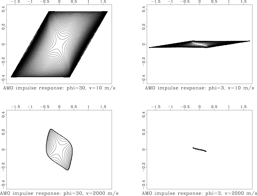
Figure 2.
The AMO impulse response traveltime. Parameters: $\left \vert{\bf h1}\right \vert=1000$ m, $\left \vert{\bf h2}\right \vert=750$ m, $t_1=1$ sec. The top plots illustrate the case of an unrealistically low velocity ($v=10$ m/s); on the bottom, $v=2000$ m/s. On the left side the azimuth rotation $\varphi =30^{\circ }$; on the right, $\varphi =3^{\circ }$
[pdf] [png] [scons]

The AMO operator's contours for different azimuth rotation angles are shown in Figure 2. Comparing the results for the case of an unrealistically low velocity (the top two plots in Figure 2) and the case of a realistic velocity (the bottom two plots) clearly demonstrates the gain in the reduction of the aperture size achieved by the aperture limitation. The gain is especially spectacular for small azimuths. When the azimuth rotation approaches zero, the area of the 3-D aperture monotonously shrinks to a 
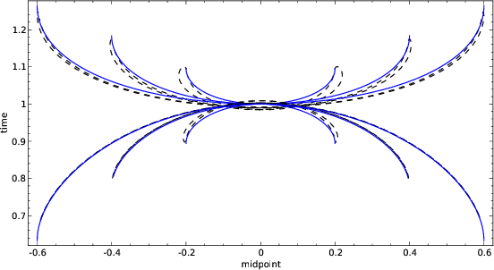
line, and the limit of the traveltime of the AMO impulse response (the inverse of (9)) approaches the offset continuation operator (14) (Figures 3). This means that taking into account the aperture limitations of AMO provides a consistent description valid for small azimuth rotations including zero (the offset continuation case). Obviously, the cost of an integral operator is proportional to its size. The size of the offset continuation operator cannot extend the difference between the offsets ${\bf
\left\vert\left\vert h_1\right\vert-\left\vert h_2\right\vert\right\vert}$. If we applied DMO and inverse DMO explicitly, the total size of the two operators would be about ${\bf\left\vert h_1\right\vert+\left\vert h_2\right\vert}$, which is substantially greater. This fact proves that in the case of small azimuth rotations the AMO price is less than those of not only 3-D prestack migration, but also 3-D DMO and inverse DMO combined (Canning and Gardner, 1992). 
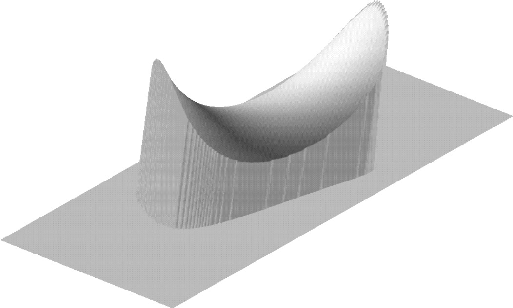
Figure 4 shows the saddle shape of the AMO operator impulse response in a 3-D AVS display.

amocom
Figure 3.
Traveltime curves of the impulse responses. The dashed lines indicate the AMO impulse response with an azimuth rotation of 3 degrees (projection on the $x$ plane); the solid lines, the 2-D offset continuation impulse response.
amocom
[pdf] [png] [sage]

amoavs
amoavs
Figure 4.
AMO impulse response traveltime in three dimensions (the AVS display). Parameters: $\left \vert{\bf h1}\right \vert=1000$ m, $\left \vert{\bf h2}\right \vert=750$ m, $t_1=1$ sec, $v=2000$ m/s, $\varphi =30^{\circ }$.
[pdf] [png]


next up previous [pdf]

Next: Conclusions Up: Fomel & Biondi: t-x Previous: CASCADING DMO AND INVERSE

2014-12-03