next up previous [pdf]

Next: Stolt stretch for anisotropic Up: EVALUATING THE PARAMETER Previous: EVALUATING THE PARAMETER

Analytic Example

A simple analytic example is the case of a constant velocity gradient. In this case the velocity distribution can be described by the linear function $ v\left(z\right)=v\left(0\right)(1+\alpha z)$ . The Stolt 
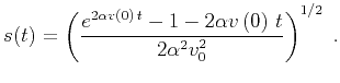
stretch transform for this case can be derived directly from equation (5) and takes the form

$\displaystyle s(t)=\left({e^{2 \alpha v\left(0\right)\,t} -1 - 2 \alpha v\left(0\right)\,t} \over {2 \alpha^2 v_0^2}\right)^{1/2}\;.$ (19)

Let $ \kappa$ be the logarithm of the velocity change $ v(z)/v(0)$ . Then 
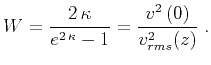
an explicit expression for $ W$ factor is found according (17) as

$\displaystyle W={{2\,\kappa}\over{e^{2\,\kappa}-1}}={v^2\left(0\right) \over v_{rms}^2(z)}\;.$ (20)

In the case of a small $ \kappa$ ', which corresponds to a small depth or a small velocity gradient, $ W \approx 1-\kappa$ . In the case of a large $ \kappa$ , $ W$ monotonically approaches zero. Equation (20) can be a useful rule of thumb for a rough estimation of $ W$ .


next up previous [pdf]

Next: Stolt stretch for anisotropic Up: EVALUATING THE PARAMETER Previous: EVALUATING THE PARAMETER

2014-03-29