|
 |
 |
 | Evaluating the Stolt-stretch parameter |  |
![[pdf]](icons/pdf.png) |
Next: EVALUATING THE PARAMETER
Up: Evaluating the Stolt-stretch parameter
Previous: Introduction
In order to simplify the references, we start with definitions of the
Stolt migration method. The reader familiar with the Stolt stretch
theory can skip this section and go on to new theoretical results in
the next section.
The basic migration theory reduces post-stack migration to a two-stage
process. The first stage is a downward continuation of the wavefield
in depth  based on the wave equation
 |
(1) |
The second stage is the imaging condition  (here the velocity
  is twice as small as the actual wave velocity). Stolt time migration
performs both stages in one step, applying the frequency-domain
operator
is twice as small as the actual wave velocity). Stolt time migration
performs both stages in one step, applying the frequency-domain
operator
 |
(2) |
where
 stands for the initial zero-offset (stacked)
seismic
section defined on the surface
stands for the initial zero-offset (stacked)
seismic
section defined on the surface  ,
,
 is the time-migrated section, and
  is
the vertical traveltime
is
the vertical traveltime
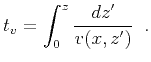 |
(3) |
The function
 in (2)
corresponds to the dispersion relation of the wave equation
(1) and in the constant velocity case has the explicit
expression
in (2)
corresponds to the dispersion relation of the wave equation
(1) and in the constant velocity case has the explicit
expression
 sign sign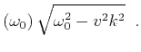 |
(4) |
The choice of the sign in equation (4) is essential
for distinguishing between upgoing and downgoing waves. The upgoing
part of the wavefield is the one used in migration.
The case of a varying velocity complicates the frequency-domain
algorithm and therefore requires special consideration.
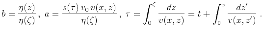
Stolt (1978) suggested the following change of the
time variable (referred to in the literature as Stolt stretch):
 |
(5) |
where  is an arbitrarily chosen constant velocity, and
  is a
function defined by the parametric expressions
is a
function defined by the parametric expressions
 |
(6) |
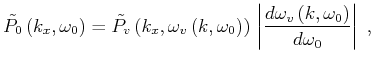
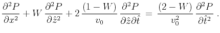
Applying equation (5),we can connect seismic time migration
to the transformed wave equation
 |
(7) |
The variables  and
and  correspond to the transformed
depth and time coordinates, which possess the following property: if
correspond to the transformed
depth and time coordinates, which possess the following property: if
 ,
,
 , and if
  ,
,
 .
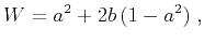
.  is a varying coefficient defined
as
is a varying coefficient defined
as
 |
(8) |
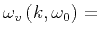
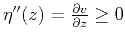
where
Since the
parameter varies slowly with  and
, Stolt
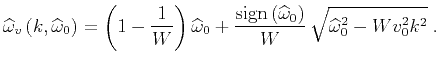
suggested to replace it with its average value. Thus equation
(7) is then approximated by an equation with constant
coefficients, which has the dispersion relation
and
, Stolt
suggested to replace it with its average value. Thus equation
(7) is then approximated by an equation with constant
coefficients, which has the dispersion relation
 |
(9) |
As outlined above, Stolt's approximate method for migration in
heterogeneous media consists of the following steps:
- stretching the time variable according to equation
(5),
- interpolating the stretched time to a regular grid,
- double Fourier transform,
- f-k time migration by the operator (2) with
the dispersion relation (9),
- inverse Fourier transform,
- inverse stretching (that is, shrinking) of the vertical time
variable on the migrated section.
The value of
must be chosen prior to migration. According to
Stolt's original definition (8),
the depth variable
gradually changes in the migration process from
zero to  , causing the coefficient
 in (8) to change monotonically from 0 to 1. If the velocity
monotonically increases with depth, then
in (8) to change monotonically from 0 to 1. If the velocity
monotonically increases with depth, then
 , and the average value of
is
, and the average value of
is
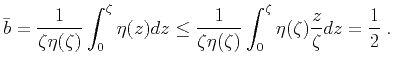 |
(10) |
As follows from equations (8) and (10),
in the case of monotonically increasing velocity, the average value of
has to be less than 1 (
equals 1 in a constant-velocity case).
Analogously, in the case of a monotonically decreasing velocity,
is always greater than 1. In practice,
is included in migration
routines as a user-defined parameter, and its value is usually chosen
to be somewhere in the range of 1/2 to 1. The next section describes a
straightforward way to determine the most appropriate value of
for
a given velocity distribution.
A useful tool for that purpose is Levin's equation for the traveltime
curve. Levin (1985) applied the stationary
phase technique to the dispersion relation (9) to
obtain an explicit equation for the summation curve of the integral
migration operator analogous to the Stolt stretch migration. The
equation evaluates the summation path in the stretched coordinate
system, as follows:
 |
(11) |
where  is the midpoint location on a zero-offset seismic section,
and
is the space coordinate on the migrated section. Equation
(11) shows that, with the stretch of the time coordinate,
the summation curve has the shape of a hyperbola with the apex at
is the midpoint location on a zero-offset seismic section,
and
is the space coordinate on the migrated section. Equation
(11) shows that, with the stretch of the time coordinate,
the summation curve has the shape of a hyperbola with the apex at
 and the center (the intersection
of the asymptotes) at
and the center (the intersection
of the asymptotes) at
 . In the case of
homogeneous media,
. In the case of
homogeneous media,  ,
,
 , and
equation (11) reduces to the known expression for a
hyperbolic diffraction traveltime curve. It is interesting to note
that inverting equation (11) for
, and
equation (11) reduces to the known expression for a
hyperbolic diffraction traveltime curve. It is interesting to note
that inverting equation (11) for
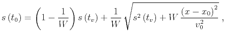
 determines the impulse response of the migration operator:
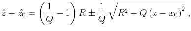 |
(12) |
where
 , and
, and  . Equation (12) can be
interpreted as the wavefront from a point source in the
. Equation (12) can be
interpreted as the wavefront from a point source in the
 domain of equation (7).
Wavefronts from a point source in the stretched coordinates for
domain of equation (7).
Wavefronts from a point source in the stretched coordinates for  have an elliptic shape, with the center of the ellipse at
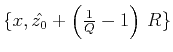 and the semi-axes
 and
and
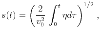
 . The ellipses stretch
differently for
. The ellipses stretch
differently for  and
and  , as shown in Figure 1.
In the upper part that corresponds to the upgoing waves, the ellipses
look nearly spherical, since the radius of the front curvature at the
top apex equals the distance from the source.
, as shown in Figure 1.
In the upper part that corresponds to the upgoing waves, the ellipses
look nearly spherical, since the radius of the front curvature at the
top apex equals the distance from the source.

|
|---|
stofro
Figure 1. Wavefronts from a point source
in the stretched coordinate system. Left: velocity decreases with
depth (W=1.5). Right: velocity increases with depth (W=0.5).
|
|---|
![[png]](icons/viewmag.png) ![[sage]](icons/sage.png)
|
|---|
|
|
|
|
| Evaluating the Stolt-stretch parameter | |
|
Next: EVALUATING THE PARAMETER
Up: Evaluating the Stolt-stretch parameter
Previous: Introduction
2014-03-29