|
|
|
|
Solution steering with space-variant filters |
Another possible application for using recursive
steering filters is to interpolate
seismic data. As an initial test
we chose to interpolate
a shot gather. We used a ![]() velocity function to construct
hyperbolic trajectories, which in turn were used to
construct our dip
field (similar to the seismic dips used in the previous section).
velocity function to construct
hyperbolic trajectories, which in turn were used to
construct our dip
field (similar to the seismic dips used in the previous section).
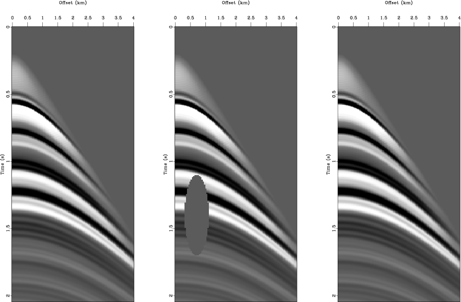
For a first test
we created a synthetic shot gather using a ![]() model as input
to a finite difference code. We then cut
a hole in this shot gather and attempted
to recover the removed values.
As Figure 7 shows we did a good job
recovering the amplitude within a few iterations.
model as input
to a finite difference code. We then cut
a hole in this shot gather and attempted
to recover the removed values.
As Figure 7 shows we did a good job
recovering the amplitude within a few iterations.
|
|---|
|
combo
Figure 7. |
|
|
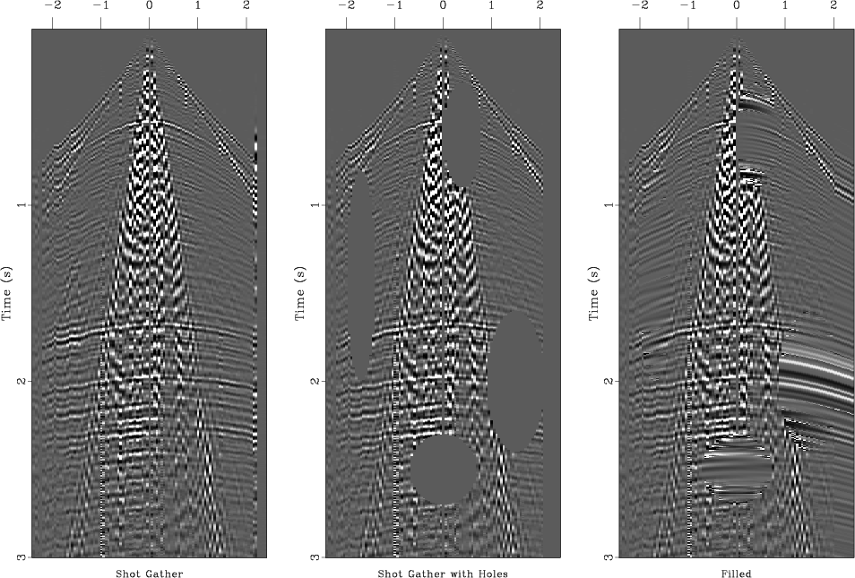
To see how the method reacted when it was given data that did not
fit its model (in this case hyperbolic moveout) we used a dataset with
significant noise problems (ground roll, bad traces, etc.). Using
the same technique as in Figure 7
we ended up with a result which did a fairly
decent job fitting portions of the data where noise content was low,
but a poor job elsewhere (Figure 8). Even where
the method did the best job of reconstructing the data, it still left
a visible footprint. A more esthetically pleasing result can be achieved
by using the above method followed a more traditional interpolation problem
using the operator ![]() and the fitting goal
and the fitting goal
|
|---|
|
wz-combo
Figure 8. Top left, original shot gather; top right, gather with holes (input); bottom left, result applying equation 18, bottom right, result after applying equation (18) followed by (19). |
|
|
|
|
|
|
Solution steering with space-variant filters |