|
|
|
|
Seismic reflection data interpolation with differential offset and shot continuation |
Missing or under-sampled shot records are a common example of data
irregularity (Crawley, 2000). The offset continuation
approach can be easily modified to work in the shot record domain.
With the change of variables ![]() , where
, where ![]() is the shot
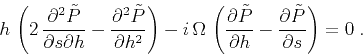
location, the frequency-domain equation (1) transforms to
the equation
is the shot
location, the frequency-domain equation (1) transforms to
the equation
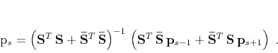
Let us consider the problem of doubling the shot density. If we use
two neighboring shot records to find the missing record between
them, the problem reduces to the least-squares system
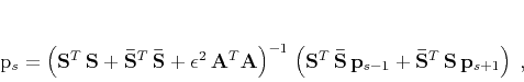
Sometimes, two neighboring shot gathers do not fully constrain the
intermediate shot. In order to add an additional constraint, I
include a regularization term in equation (16), as
follows:
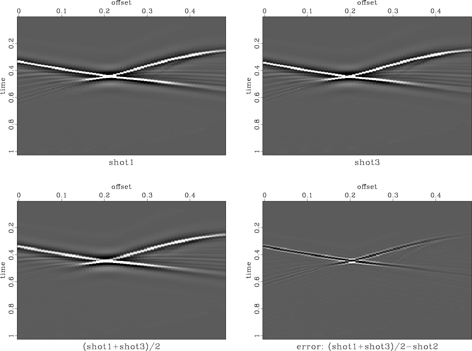
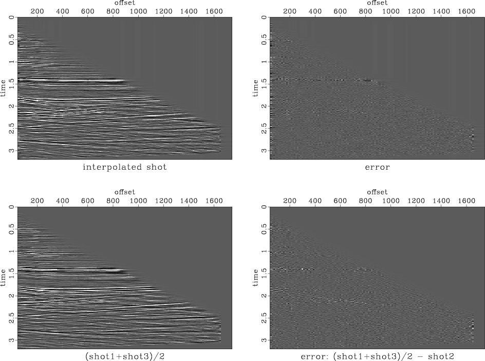
Figure 9 shows the result of a shot interpolation experiment using the constant-velocity synthetic from Figure 4. In this experiment, I removed one of the shot gathers from the original NMO-corrected data and interpolated it back using equation (17). Subtracting the true shot gather from the reconstructed one shows a very insignificant error, which is further reduced by using the PEF regularization (right plots in Figure 9). The two neighboring shot gathers used in this experiment are shown in the top plots of Figure 8. For comparison, the bottom plots in Figure 8 show the simple average of the two shot gathers and its corresponding prediction error. As expected, the error is significantly larger than the error of shot continuation. An interpolation scheme based on local dips in the shot direction would probably achieve a better result, but it is significantly more expensive than the shot continuation scheme introduced above.
|
|---|
|
shot3
Figure 8. Top: Two synthetic shot gathers used for the shot interpolation experiment. An NMO correction has been applied. Bottom: simple average of the two shot gathers (left) and its prediction error (right). |
|
|

|
|---|
|
shotin
Figure 9. Synthetic shot interpolation results. Left: interpolated shot gathers. Right: prediction errors (the differences between interpolated and true shot gathers), plotted on the same scale. |
|
|
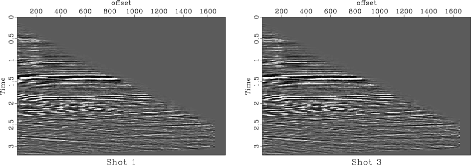
A similar experiment with real data from a North Sea marine dataset is reported in Figure 11. I removed and reconstructed a shot gather from the two neighboring gathers shown in Figure 10. The lower parts of the gathers are complicated by salt dome reflections and diffractions with conflicting dips. The simple average of the two input shot gathers (bottom plots in Figure 11) works reasonably well for nearly flat reflection events but fails to predict the position of the back-scattered diffractions events. The shot continuation method works well for both types of events (top plots in Figure 11). There is some small and random residual error, possibly caused by local amplitude variations.
|
|---|
|
elfshot3
Figure 10. Two real marine shot gathers used for the shot interpolation experiment. An NMO correction has been applied. |
|
|
|
|---|
|
elfshotin
Figure 11. Real-data shot interpolation results. Top: interpolated shot gather (left) and its prediction error (right). Bottom: simple average of the two input shot gathers (left) and its prediction error (right). |
|
|
Analogously to the case of offset continuation, it is possible to extend the shot continuation method to three dimensions. A simple modification of the proposed technique would also allow us to use more than two shot gathers in the input or to extrapolate missing shot gathers at the end of survey lines.
|
|
|
|
Seismic reflection data interpolation with differential offset and shot continuation |
![\begin{displaymath}
\widehat{\widehat{P}}(s_2) = \widehat{\widehat{P}}(s_1)\,
...
...right)\,
\frac{k_h\,h-\Omega}{2\,k_h\,h-\Omega}\right]}\;,
\end{displaymath}](img41.png)
![\begin{displaymath}
\left[\begin{array}{c}
\mathbf{S} \\
\mathbf{\bar{S}}
...
...s-1} \\
\mathbf{S}\,\mathbf{p}_{s+1}
\end{array}\right]\;,
\end{displaymath}](img46.png)