Seismic reflection data interpolation with differential offset and shot continuation

Constant-velocity synthetic

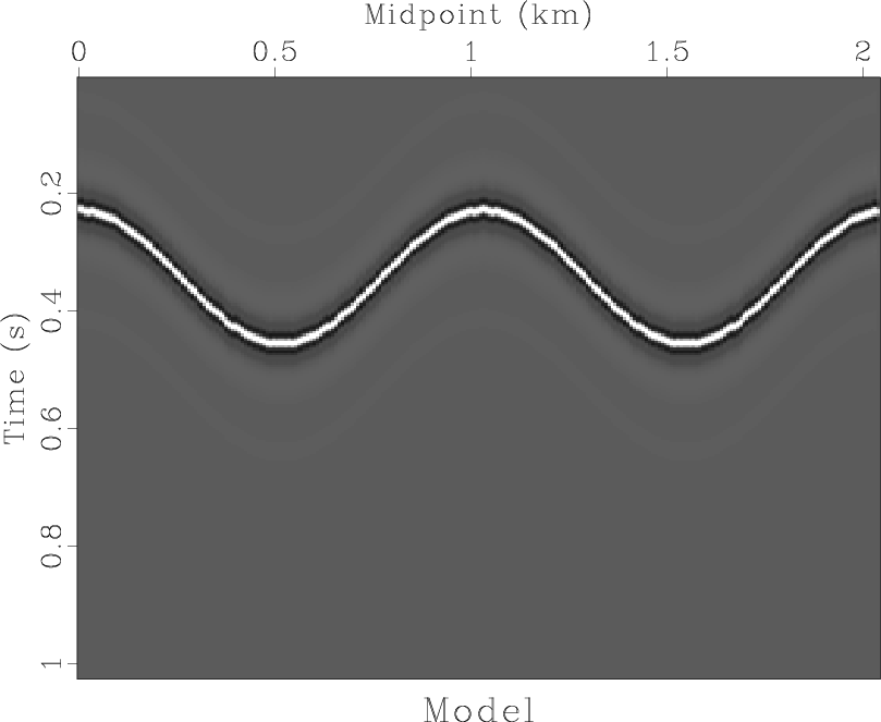
cup Figure 3. Reflector model for the constant-velocity test

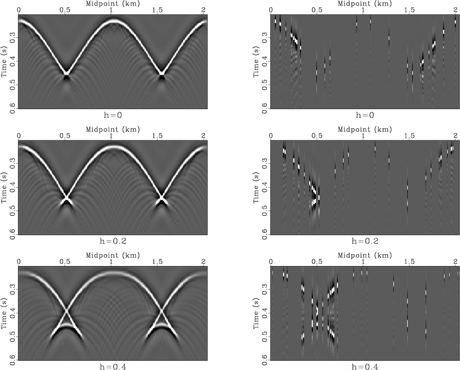
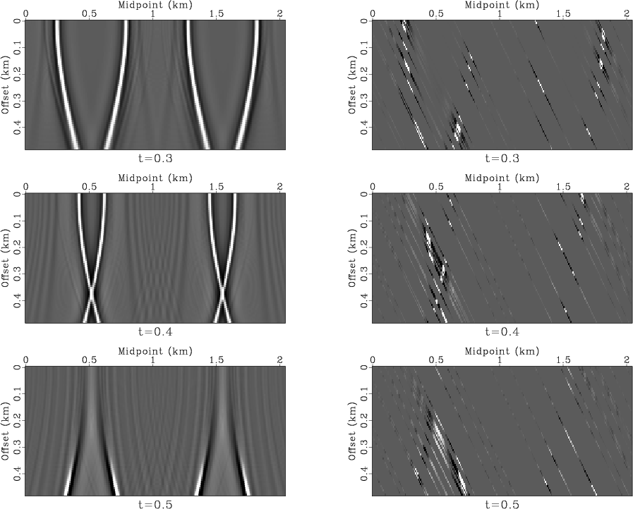
A sinusoidal reflector shown in Figure 3 creates complicated reflection data, shown in Figures 4 and 5. To set up a test for regularization by offset continuation, I removed 90% of randomly selected shot gathers from the input data. The syncline parts of the reflector lead to traveltime triplications at large offsets. A mixture of different dips from the triplications would make it extremely difficult to interpolate the data in individual common-offset gathers, such as those shown in Figure 4. The plots of time slices after NMO (Figure 5) clearly show that the data are also non-stationary in the offset direction. Therefore, a simple offset interpolation scheme is also doomed.

data
Figure 4. Prestack common-offset gathers for the constant-velocity test. Left: ideal data (after NMO). Right: input data (90% of shot gathers removed). Top, center, and bottom plots correspond to different offsets.

tslice
Figure 5. Time slices of the prestack data for the constant-velocity test. Left: ideal data (after NMO). Right: input data (90% of random gathers removed). Top, center, and bottom plots correspond to time slices at 0.3, 0.4, and 0.5 s.

Figure 6 shows the reconstruction process on individual frequency slices. Despite the complex and non-stationary character of the reflection events in the frequency domain, the offset continuation equation is able to accurately reconstruct them from the decimated data.

fslice
Figure 6. Interpolation in frequency slices. Left: input data (90% of the shot gathers removed). Right: interpolation output. Top, bottom, and middle plots correspond to different frequencies. The real parts of the complex-valued data are shown.

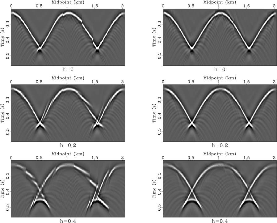
Figure 7 shows the result of interpolation after the data are transformed back to the time domain. The offset continuation result (right plots in Figure 7) reconstructs the ideal data (left plots in Figure 4) very accurately even in the complex triplication zones, while the result of simple offset interpolation (left plots in Figure 7) fails as expected. The simple interpolation scheme applied the offset derivative $\frac{\partial}{\partial h}$ in place of the offset continuation equation and thus did not take into account the movement of the events across different midpoints.

all
Figure 7. Interpolation in common-offset gathers. Left: output of simple offset interpolation. Right: output of offset continuation interpolation. Compare with Figure 4. Top, center, and bottom plots correspond to different common-offset gathers.

The constant-velocity test results allow us to conclude that, when all the assumptions of the offset continuation theory are met, it provides a powerful method of data regularization.

Being encouraged by the synthetic results, I proceed to a three-dimensional real data test.

Analogously to integral azimuth moveout operator (Biondi et al., 1998), differential offset continuation can be applied in 3-D for regularizing seismic data prior to prestack imaging.

In the next section, I return to the 2-D case to consider an important problem of shot gather interpolation.

Seismic reflection data interpolation with differential offset and shot continuation