 |
 |
 |
 | Traveltime computation with
the linearized eikonal equation |  |
![[pdf]](icons/pdf.png) |
Next: About this document ...
Up: Fomel: Linearized Eikonal
Previous: ACKNOWLEDGMENTS
-
Alkhalifah, T., 1997, Acoustic approximations for processing in transversely
isotropic media: submitted to Geophysics.
-
-
Biondi, B., 1992, Solving the frequency-dependent eikonal equation: 62nd Ann.
Internat. Mtg, Soc. of Expl. Geophys., 1315-1319.
-
-
Fowler, P. J., 1994, Finite-difference solutions of the 3-D eikonal equation
in spherical coordinates: 64th Ann. Internat. Mtg, Soc. of Expl. Geophys.,
1394-1397.
-
-
Gray, S. H., and W. P. May, 1994, Kirchhoff migration using eikonal equation
traveltimes: Geophysics, 59, 810-817.
-
-
Lavrentiev, M. M., V. G. Romanov, and V. G. Vasiliev, 1970, Multidimensional
inverse problems for differential equations: Springer-Verlag, volume 167 of Lecture Notes in Mathematics.
-
-
Nichols, D. E., 1994, Imaging complex structures using band-limited Green's
functions: PhD thesis, Stanford University.
-
-
Popovici, M., 1991, Finite difference travel time maps, in SEP-70:
Stanford Exploration Project, 245-256.
-
-
Schneider, W. A., 1995, Robust and efficient upwind finite-difference
traveltime calculations in three dimensions: Geophysics, 60,
1108-1117.
-
-
van Trier, J., and W. W. Symes, 1991, Upwind finite-difference calculation of
traveltimes: Geophysics, 56, 812-821.
-
-
Cerveny, V., I. A. Molotkov, and I. Pšencik., 1977, Ray method in
seismology: Univerzita Karlova.
-
-
Vidale, J. E., 1990, Finite-difference calculation of traveltimes in three
dimensions: Geophysics, 55, 521-526.
-
Appendix
A
A SIMPLE derivation of the eikonal and transport equations
In this Appendix, I remind the reader how the eikonal equation is
derived from the wave equation. The derivation is classic and can be
found in many popular textbooks. See, for example, (Cerveny et al., 1977).
Starting from the wave equation,
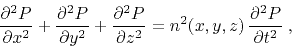 |
(8) |
we introduce a trial solution of the form
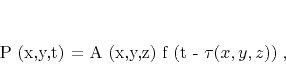 |
(9) |
where  is the eikonal, and
  is the wave amplitude. The
waveform function
is the wave amplitude. The
waveform function  is assumed to be a high frequency
(discontinuous) signal. Substituting solution (F-2) into
equation (F-1), we arrive at the constraint
is assumed to be a high frequency
(discontinuous) signal. Substituting solution (F-2) into
equation (F-1), we arrive at the constraint
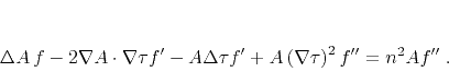 |
(10) |
Here
 denotes the Laplacian operator.
Equation (F-3) is as exact as the initial wave equation
(F-1) and generally difficult to satisfy. However, we can
try to satisfy it asymptotically, considering each of the
high-frequency asymptotic components separately. The leading-order
component corresponds to the second derivative of the wavelet
denotes the Laplacian operator.
Equation (F-3) is as exact as the initial wave equation
(F-1) and generally difficult to satisfy. However, we can
try to satisfy it asymptotically, considering each of the
high-frequency asymptotic components separately. The leading-order
component corresponds to the second derivative of the wavelet  .
Isolating this component, we find that it is satisfied if and only if
the traveltime function
.
Isolating this component, we find that it is satisfied if and only if
the traveltime function  satisfies the eikonal equation
(1).
satisfies the eikonal equation
(1).
The next asymptotic order corresponds to the first derivative  . It
leads to the amplitude transport equation
. It
leads to the amplitude transport equation
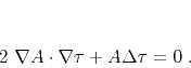 |
(11) |
The amplitude, defined by equation (F-4), is often referred
to as the amplitude of the zero-order term in the ray series. A series
expansion of the function in high-frequency asymptotic components
produces recursive differential equations for the terms of higher
order. In practice, equation (F-4) is sufficiently accurate
for describing the major amplitude trends in most of the cases. It
fails, however, in some special cases, such as caustics and diffraction.
Appendix
B
CONNECTION OF THE LINEARIZED EIKONAL EQUATION AND
TRAVELTIME TOMOGRAPHY
The eikonal equation (1) can be rewritten in the form
 |
(12) |
where  is the unit vector, pointing in the traveltime
gradient direction. The integral solution of equation (G-1)
takes the form
is the unit vector, pointing in the traveltime
gradient direction. The integral solution of equation (G-1)
takes the form
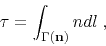 |
(13) |
which states that the traveltime can be computed by
integrating the slowness  along the ray
 ,
tangent at every point to the gradient direction .
,
tangent at every point to the gradient direction .
Similarly, we can rewrite the linearized eikonal equation (5)
in the form
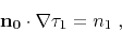 |
(14) |
where  is the unit vector, pointing in gradient
direction for the initial traveltime
is the unit vector, pointing in gradient
direction for the initial traveltime  . The integral solution
of equation (G-3) takes the form
. The integral solution
of equation (G-3) takes the form
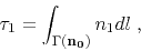 |
(15) |
which states that the traveltime perturbation  can be
computed by integrating the slowness perturbation
can be
computed by integrating the slowness perturbation  along the
ray
along the
ray
 , defined by the initial slowness model
 . This is exactly the basic principle of traveltime
tomography.
. This is exactly the basic principle of traveltime
tomography.
I have borrowed this proof from Lavrentiev et al. (1970), who used linearization
of the eikonal equation as the theoretical basis for traveltime inversion.
|
|
|
|
| Traveltime computation with
the linearized eikonal equation | |
|
Next: About this document ...
Up: Fomel: Linearized Eikonal
Previous: ACKNOWLEDGMENTS
2013-03-03