Traveltime computation with the linearized eikonal equation

Discussion

Although the first numerical experiments have been too incomplete for drawing any solid conclusions, it is interesting to discuss the possible applications of the linearized eikonal.

Multi-valued traveltimes

Conventional eikonal solvers usually force the choice of a particular branch of the multi-valued traveltime, most commonly the first-arrival branch. However, in some cases other branches may in fact be more useful for imaging or velocity estimation (Gray and May, 1994). When the linearization assumption is correct, the linearized eikonal should follow the branch of the initial traveltime. This branch does not have to be the first arrival. It can correspond to any other arrival, such as reflected waves or multiple reflections.

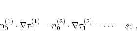
Spherical Coordinates

Though the eikonal equation itself does not favor any particular direction, its solution for the case of a point source lands more naturally into a spherical coordinate system. van Trier and Symes (1991), Popovici (1991), Fowler (1994), and Schneider (1995) presented upwind finite-difference eikonal schemes based on a spherical computational grid. To use the linearized equation (5) on such a grid, it is necessary to rewrite the gradient operator in the spherical coordinates, as follows:

$$\nabla \tau = \left\{ \frac{\partial \tau}{\partial r} ,\... ...\sin^2 \theta} \frac{\partial \tau}{\partial \phi}\right\}\;.$$

.

Interpolation

One of the most natural applications for the linearized eikonal is interpolation of traveltimes. Interpolating regularly gridded input (such as subsampled traveltime tables) reduces to masked inversion of equation (5). Interpolating irregular input (such as the result of a ray tracing procedure) reduces to regularized inversion. In both cases, a simpler way of traveltime binning would be required to initiate the linearization.

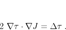
Tomography

Tomographic velocity estimation is possible when the input traveltime data corresponds to a collection of sources. In this case, we can reduce the linearized traveltime inversion to the system of equations

$$n_0^{(1)} \cdot \nabla \tau_1^{(1)} = n_0^{(2)} \cdot \nabla \tau_1^{(2)} = \cdots = s_1\;.$$ (6)

Here $\tau_1^{(i)}$ stands for the traveltime from source $i$. Equations (6) are additionally constrained by the known values of the traveltime fields at the receiver locations.

Amplitudes

The amplitude transport equation, briefly reviewed in Appendix A, has the form (F-4). Introducing the logarithmic amplitude 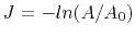$J = - ln (A/A_0)$, where $A_0$ is the constant reference, we can rewrite this equation in the form

$$2 \nabla \tau \cdot \nabla J = \Delta \tau\;.$$ (7)

The left-hand side of equation (7) has exactly the same form as the left-hand side part of the linearized eikonal equation (5). This suggests reusing the traveltime computation scheme for amplitude calculations. The amplitude transport equation is linear. However, it explicitly depends on the traveltime. Therefore, the amplitude computation needs to be coupled with the eikonal solution.

Anisotropy

In a recent paper, Alkhalifah (1997) proposed a simple eikonal-type equation for seismic imaging in vertically transversally-isotropic media. Alkhalifah's equation should be suitable for linearization, either in the normal moveout velocity $V_{NMO}$ or in the dimensionless anisotropy parameter $\eta$. This untested opportunity looks promising because of the validity of the weak anisotropy assumption in many regions of the world.

Traveltime computation with the linearized eikonal equation