|
|
|
|
Exploring three-dimensional implicit wavefield extrapolation with the helix transform |
The major obstacle of applying an implicit extrapolation in three
dimensions is that the inverted matrix is no longer tridiagonal. If we
approximate the second derivative (Laplacian) on the 2-D plane with
the commonly used five-point filter
![]() , then the matrix on the left side of equation
(14), under the usual mapping of vectors from a
two-dimensional mesh to one dimension, takes the infamous
blocked-tridiagonal form (Birkhoff, 1971)
, then the matrix on the left side of equation
(14), under the usual mapping of vectors from a
two-dimensional mesh to one dimension, takes the infamous
blocked-tridiagonal form (Birkhoff, 1971)
A helix transform, recently proposed by one of the authors
(Claerbout, 1997a), sheds new light on this old problem.
Let us assume that the extrapolation filter is applied by sliding it
along the ![]() direction in the
direction in the ![]() plane. The diagonal
discontinuities in matrix
plane. The diagonal
discontinuities in matrix
![]() occur exactly in the
places where the forward leg of the filter slides outside the
computational domain. Let's imagine a situation, where the leg of the
filter that went to the end of the
occur exactly in the
places where the forward leg of the filter slides outside the
computational domain. Let's imagine a situation, where the leg of the
filter that went to the end of the ![]() column, would immediately
appear at the beginning of the next column. This situation defines a
different mapping from two computational dimensions to the one
dimension of linear algebra. The mapping can be understood as the
helix transform, illustrated in Figure
column, would immediately
appear at the beginning of the next column. This situation defines a
different mapping from two computational dimensions to the one
dimension of linear algebra. The mapping can be understood as the
helix transform, illustrated in Figure ![]() and explained
in detail by Claerbout (1997a). According to this
transform, we replace the original two-dimensional filter with a long
one-dimensional filter. The new filter is partially filled with zero
values (corresponding to the back side of the helix), which can be
safely ignored in the convolutional computation.
and explained
in detail by Claerbout (1997a). According to this
transform, we replace the original two-dimensional filter with a long
one-dimensional filter. The new filter is partially filled with zero
values (corresponding to the back side of the helix), which can be
safely ignored in the convolutional computation.
|
|---|
|
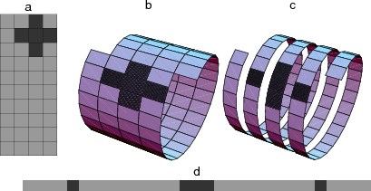
helix
Figure 4. The helix transform of two-dimensional filters to one dimension. The two-dimensional filter in the left plot is equivalent to the one-dimensional filter in the right plot, assuming that a shifted periodic condition is imposed on one of the axes. |
|
|
This is exactly the helix transform that is required to make all the
diagonals of matrix
![]() continuous. In the case of
laterally invariant coefficients, the matrix becomes strictly Toeplitz
(having constant values along the diagonals) and represents a
one-dimensional convolution on the helix surface. Moreover, this
simplified matrix structure applies equally well to larger
second-derivative filters ( such as those described in Appendix B),
with the obvious increase of the number of Toeplitz diagonals.
Inverting matrix
continuous. In the case of
laterally invariant coefficients, the matrix becomes strictly Toeplitz
(having constant values along the diagonals) and represents a
one-dimensional convolution on the helix surface. Moreover, this
simplified matrix structure applies equally well to larger
second-derivative filters ( such as those described in Appendix B),
with the obvious increase of the number of Toeplitz diagonals.
Inverting matrix
![]() becomes once again a simple
inverse filtering problem. To decompose the 2-D filter into a pair
consisting of a causal minimum-phase filter and its adjoint, we can
apply spectral factorization methods from the 1-D filtering theory
(Claerbout, 1992,1976), for example,
Kolmogorov's highly efficient method (Kolmogorov, 1939). Thus, in the case
of a laterally invariant implicit extrapolation, matrix inversion
reduces to a simple and efficient recursive filtering, which we need
to run twice: first in the forward mode, and second in the adjoint
mode.
becomes once again a simple
inverse filtering problem. To decompose the 2-D filter into a pair
consisting of a causal minimum-phase filter and its adjoint, we can
apply spectral factorization methods from the 1-D filtering theory
(Claerbout, 1992,1976), for example,
Kolmogorov's highly efficient method (Kolmogorov, 1939). Thus, in the case
of a laterally invariant implicit extrapolation, matrix inversion
reduces to a simple and efficient recursive filtering, which we need
to run twice: first in the forward mode, and second in the adjoint
mode.
|
|---|
|
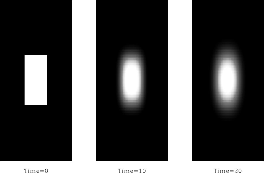
heat3d
Figure 5. Heat extrapolation in two dimensions, computed by an implicit scheme with helix recursive filtering. The left plot shows the input temperature distributions; the two other plots, the extrapolation result at different time steps. The coefficient |
|
|
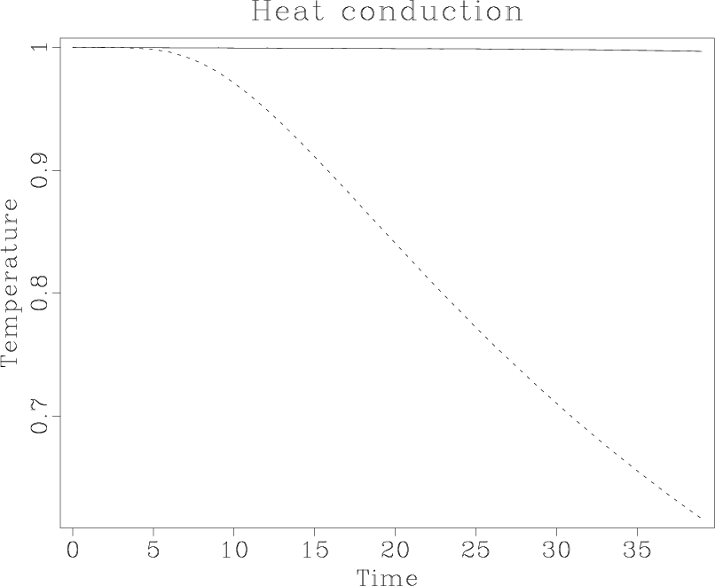
Figure 5 shows the result of applying the helix transform to an implicit heat extrapolation of a two-dimensional temperature distribution. The unconditional stability properties are nicely preserved, which can be verified by examining the plot of changes in the average temperature (Figure 6).
|
heat-mean
Figure 6. Demonstration of the stability of implicit extrapolation. The solid curve shows the normalized mean temperature, which remains nearly constant throughout the extrapolation time. The dashed curve shows the normalized maximum value, which exhibits the expected Gaussian shape. |
|
|---|---|
|
|
In principle, we could also treat the case of a laterally invariant
coefficient with the help of the Fourier transform. Under what
circumstances does the helix approach have an advantage over Fourier
methods? One possible situation corresponds to a very large input data
size with a relatively small extrapolation filter. In this case, the
![]() cost of the fast Fourier transform is comparable with the
cost of the fast Fourier transform is comparable with the
![]() cost of the space-domain deconvolution (where
cost of the space-domain deconvolution (where ![]() corresponds to the data size, and
corresponds to the data size, and ![]() is the filter size). Another
situation is when the boundary conditions of the problem have an
essential lateral variation. The latter case may occur in applications
of velocity continuation, which we discuss in the next section. Later
in this paper, we return to the discussion of problems associated with
lateral variations.
is the filter size). Another
situation is when the boundary conditions of the problem have an
essential lateral variation. The latter case may occur in applications
of velocity continuation, which we discuss in the next section. Later
in this paper, we return to the discussion of problems associated with
lateral variations.
|
|
|
|
Exploring three-dimensional implicit wavefield extrapolation with the helix transform |
![\begin{displaymath}
\tilde{\mathbf{A}} = \left(\mathbf{I} -c\,\mathbf{D}_2\righ...
...& & -c_{n} \,\mathbf{I} &
\mathbf{A}_n
\end{array}\right]\;.
\end{displaymath}](img60.png)