Madagascar tutorial

Making synthetic data

cmp
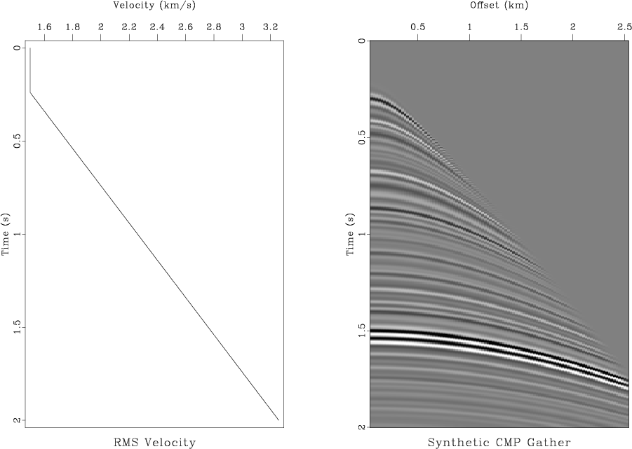
Figure 1. RMS velocity profile (left) and synthetic CMP gather (right).

cmp2
Figure 2. RMS velocity profiles for primaries and multiples (left) and synthetic multiple-infected CMP gather (right).

nmo
Figure 3. Semblance scan (left) and NMO with the primary velocity (right) applied to the synthetic CMP gather from Figure 2.

1. Change directory to ../synth.

2. We will start by generating a synthetic CMP (common midpoint) gather using a linearly increasing RMS (root-mean-square) velocity, a random reflectivity, and a Ricker wavelet (Figure 1). To display this figure on your screen, run

   bash$ scons cmp.view
   

   You can examine the SConstruct file to see the programs and parameter selections for generating these data. What does sfinmo do?

3. Next, we add some regular noise to the gather in the form of multiple reflections. In a rough approximation, the velocity trend of surface-related pegleg multiples follows that of the primary reflections but with a delay by the time of the water-bottom reflection (Figure 2.) To reproduce the figure on your screen, run

   bash$ scons cmp2.view
   

4. To better understand the effect of multiples on the data, we can examine the result of velocity analysis by semblance scanning and NMO (normal moveout) correction using the velocity of the primary reflection (Figure 3.) NMO flattens primary reflections and highlights multiple reflections as curved events. In processing field data, we may not know the primary velocity precisely and would need to estimate it.

5. CHALLENGE 1: The modeled synthetic data uses rough approximations. Your first challenge is to try making it more realistic or more challenging. You can modify the SConstruct file to change parameters (such as the water depth), to add noise (check out sfnoise), amplitude variations with offset, other kinds of multiples, etc.

from rsf.proj import *

t0 = 0.24 # water depth in two-way time

# RMS velocity profile
Flow('vel',None,
     '''
     math n1=501 d1=0.004 output=1.5+x1-%g
     label1=Time unit1=s | clip2 lower=1.5
     ''' % t0)
Plot('vel',
     '''
     graph title="RMS Velocity" transp=y yreverse=y
     label2=Velocity unit2=km/s wheretitle=b wherexlabel=t
     ''')

# Synthetic CMP gather
Flow('trace','vel',
     '''
     noise rep=y seed=2016 | math output=input^3 |
     cut max1=%g | ricker1 frequency=20
     ''' % t0)
Flow('cmp','trace vel',
     '''
     spray axis=2 n=100 o=0.05 d=0.025 label=Offset unit=km |
     inmo half=n velocity=${SOURCES[1]} | mutter half=n v0=1.5
     ''')
Plot('cmp','grey title="Synthetic CMP Gather" ')

Result('cmp','vel cmp','SideBySideAniso')

# First pegleg multiple
Flow('vel1','vel',
     '''
     math n1=501 d1=0.004 output=1.5+x1-%g
     label1=Time unit1=s | clip2 lower=1.5
     ''' % (2*t0))
Flow('trace1','trace',
     '''
     pad beg1=%d | window n1=501 |
     scale dscale=-0.5
     ''' % int(t0/0.004))
Flow('mult1','trace1 vel1',
     '''
     spray axis=2 n=100 o=0.05 d=0.025 label=Offset unit=km |
     inmo half=n velocity=${SOURCES[1]} | mutter half=n v0=1.5
     ''')

# Second pegleg multiple
Flow('vel2','vel1',
     '''
    math n1=501 d1=0.004 output=1.5+x1-%g
    label1=Time unit1=s | clip2 lower=1.5
    ''' % (3*t0))
Flow('trace2','trace1',
     '''
     pad beg1=%d | window n1=501 |
     scale dscale=-0.5
     ''' % int(t0/0.004))
Flow('mult2','trace2 vel2',
     '''
     spray axis=2 n=100 o=0.05 d=0.025 label=Offset unit=km |
     inmo half=n velocity=${SOURCES[1]} | mutter half=n v0=1.5
     ''')
Plot('vel2','vel vel1 vel2',
     '''
     cat axis=2 ${SOURCES[1:3]} |
     graph title="RMS Velocity" transp=y yreverse=y dash=0,1,1
     label2=Velocity unit2=km/s wheretitle=b wherexlabel=t
     ''')

Flow('cmp2','cmp mult1 mult2','add ${SOURCES[1:3]}')
Plot('cmp2','grey title="CMP Gather with Multiples" ')
Result('cmp2','vel2 cmp2','SideBySideAniso')

# Velocity analysis
Flow('vscan','cmp2',
     'vscan half=n v0=1.5 nv=101 dv=0.02 semblance=y')
Plot('vscan','grey color=j allpos=y title="Semblance Scan" ')

Flow('nmo','cmp2 vel','nmo half=n velocity=${SOURCES[1]}')
Plot('nmo','grey title="NMO with Primary Velocity" ')

Result('nmo','vscan nmo','SideBySideAniso')

End()

Madagascar tutorial