|
|
|
|
Velocity-independent |
|
|---|
|
dataP
Figure 8. |
|
|
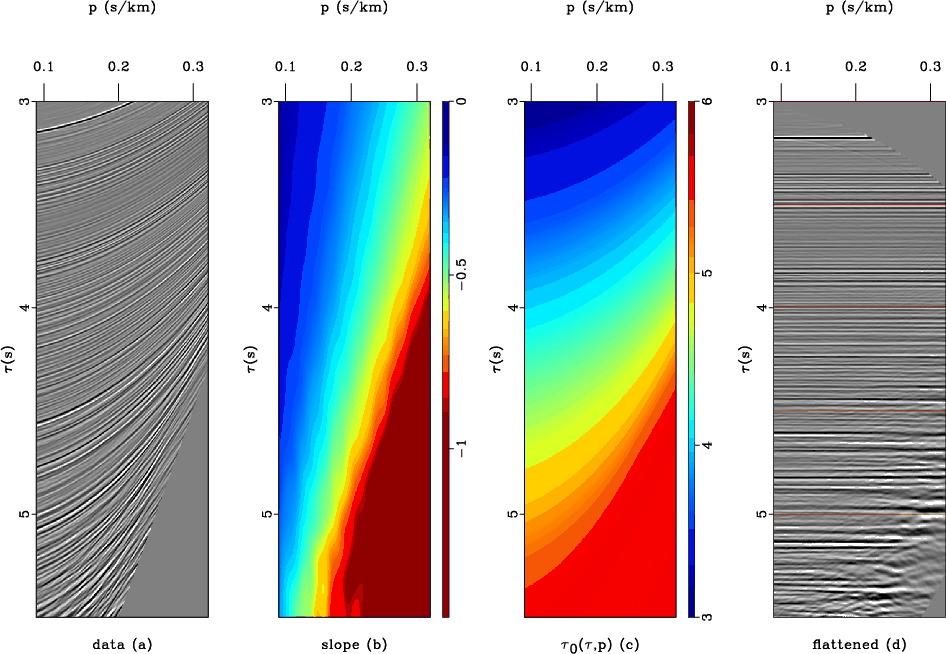
Figure 9 presents the results of the proposed ![]() -
-![]() processing on a
field data example from a marine acquisition. Figure 9a shows a
processing on a
field data example from a marine acquisition. Figure 9a shows a ![]() -
-![]() transformed CMP gather. The data are taken
from a deep water (3.5 s of sea-depth) dataset with poor offset
sampling (
transformed CMP gather. The data are taken
from a deep water (3.5 s of sea-depth) dataset with poor offset
sampling (
![]() ) that aliases the steepest seismic
events. Spatial aliasing creates artifacts in
) that aliases the steepest seismic
events. Spatial aliasing creates artifacts in ![]() -
-![]() domain that bias
the PWD slope estimate. In order to mitigate the effect of the
aliasing, we interpolated the raw data by means of an FX algorithm
(Spitz, 1991). The original trace recording is 7.0 s long but,
since the SNR decreases significantly after 5.0 s, we window the CMP
gather and process seismic events only between 3.0 and
6.0 s. The CMP maximum offset-to-depth ratio reaches 1.5 for
larger value of the horizontal slope
domain that bias
the PWD slope estimate. In order to mitigate the effect of the
aliasing, we interpolated the raw data by means of an FX algorithm
(Spitz, 1991). The original trace recording is 7.0 s long but,
since the SNR decreases significantly after 5.0 s, we window the CMP
gather and process seismic events only between 3.0 and
6.0 s. The CMP maximum offset-to-depth ratio reaches 1.5 for
larger value of the horizontal slope ![]() . As for the synthetic case,
the data should carry enough information to well resolve the
horizontal velocity and the anellipticity parameter. Figure 9b
shows the dominant local-slope
. As for the synthetic case,
the data should carry enough information to well resolve the
horizontal velocity and the anellipticity parameter. Figure 9b
shows the dominant local-slope ![]() field
automatically measure from the data using the PWD algorithm. As in
the synthetic case, we use these slopes to construct the prediction
operator that allows us to paint the zero-slope traveltime map
field
automatically measure from the data using the PWD algorithm. As in
the synthetic case, we use these slopes to construct the prediction
operator that allows us to paint the zero-slope traveltime map
![]() along the reflection events (Figure 9c). The
along the reflection events (Figure 9c). The ![]() values are finally used to unwrap the trace shifts until the gather
is completely flattened. The good alignment of the NMO corrected
traces (Figure 9d) confirms the robustness of predictive painting
with real data. Figure 10 shows spectra of the
recovered interval parameters using Fowler's equations 27
and 28. The plots are overlaid with the profiles (yellow
curves) recovered using a layer-based
values are finally used to unwrap the trace shifts until the gather
is completely flattened. The good alignment of the NMO corrected
traces (Figure 9d) confirms the robustness of predictive painting
with real data. Figure 10 shows spectra of the
recovered interval parameters using Fowler's equations 27
and 28. The plots are overlaid with the profiles (yellow
curves) recovered using a layer-based ![]() -
-![]() Dix inversion
(Ferla and Cibin, 2009) and by the profiles obtained after an automated
picking of the recovered trends. Our solution (red curves) follows
the Dix trends (yellow curves) even though it exhibits a slight
decrease in accuracy. The poor SNR for later and steeper events and
the numerical differentiation of the zero-slope traveltime
Dix inversion
(Ferla and Cibin, 2009) and by the profiles obtained after an automated
picking of the recovered trends. Our solution (red curves) follows
the Dix trends (yellow curves) even though it exhibits a slight
decrease in accuracy. The poor SNR for later and steeper events and
the numerical differentiation of the zero-slope traveltime ![]() and slope
and slope ![]() make the field data results noisier. As expected, the
high-order moveout parameters appear to be more sensitive to the
noise. Moreover, the more pronounced enlargement of the
make the field data results noisier. As expected, the
high-order moveout parameters appear to be more sensitive to the
noise. Moreover, the more pronounced enlargement of the
![]() trend in comparison with the
trend in comparison with the ![]() trend
confirms that the latter parameter is better constrained by the data
(Tsvankin, 2006).
trend
confirms that the latter parameter is better constrained by the data
(Tsvankin, 2006).

|
|---|
|
int-painting-mask
Figure 9. Parameters spectra for interval normal moveout (a), horizontal velocity (b) and anellipticity parameter |
|
|
|
|
|
|
Velocity-independent |