|
|
|
|
Velocity-independent |
As shown in Table 1, Fowler's is the only set of
equations that do not require an explicit use of the curvature
![]() . The dependence on the curvature is absorbed by the
. The dependence on the curvature is absorbed by the ![]() function. The other two sets of equations, Dix and stripping formulas,
as well as the equations for effective parameters, do need
curvature. The curvature computation can be problematic when the data
are contaminated by noise. This makes these three methods (effective,
stripping, and Dix) less practical when applied to real data with poor
SNR. However, Fowler's rules represent a way to circumvent the
problem. In fact, if we can find an algorithm that estimates the
function. The other two sets of equations, Dix and stripping formulas,
as well as the equations for effective parameters, do need
curvature. The curvature computation can be problematic when the data
are contaminated by noise. This makes these three methods (effective,
stripping, and Dix) less practical when applied to real data with poor
SNR. However, Fowler's rules represent a way to circumvent the
problem. In fact, if we can find an algorithm that estimates the ![]() mapping function directly from the data, all the curvature issues
will get solved.
mapping function directly from the data, all the curvature issues
will get solved.
The desired algorithm exists and is known as seismic image flattening. The idea of using local slopes for automatic flattening was introduced by Bienati and Spagnolini (2001) and Lomask et al. (2006). Flattening by predictive painting (appendix A) uses the local-slope field to construct a recursive prediction operator (equation A-4) that spreads a traveltime reference trace in the image and predicts the reflecting surfaces which are then unwrapped until the image is flattened.
We propose bypassing the issue of estimating the zero-slope time ![]() field by using the predictive painting
approach. Let us discuss how it works on the previously shown
synthetic data in Figure 7a.
Figure 7b shows local event slope
field by using the predictive painting
approach. Let us discuss how it works on the previously shown
synthetic data in Figure 7a.
Figure 7b shows local event slope ![]() measured from the data
using the PWD algorithm. Figure 7c shows how predictive
painting spreads a zero-slope time
measured from the data
using the PWD algorithm. Figure 7c shows how predictive
painting spreads a zero-slope time ![]() reference trace along
local data slopes to predict the zero-slope time
reference trace along
local data slopes to predict the zero-slope time ![]() mapping
field and hence the geometry of the traveltime reflection curves along
mapping
field and hence the geometry of the traveltime reflection curves along
![]() -
-![]() CMP gather. Because this procedure does not involve curvature
computations, it represents a much more robust way of obtaining the
CMP gather. Because this procedure does not involve curvature
computations, it represents a much more robust way of obtaining the
![]() field that is needed by the inversion formulas in
equations 27 and 28. After
field that is needed by the inversion formulas in
equations 27 and 28. After ![]() has been found, we also have what we need to perform gather flattening
(Burnett and Fomel, 2009a,b).
Unshifting each trace (Figure 7d) automatically flattens the
data, thus performing a velocity-independent
has been found, we also have what we need to perform gather flattening
(Burnett and Fomel, 2009a,b).
Unshifting each trace (Figure 7d) automatically flattens the
data, thus performing a velocity-independent ![]() -
-![]() NMO correction. As
expected, all events are perfectly aligned, and the correction does
not suffer from instabilities of curvature estimation. Moreover,
predictive painting is automatic and does not require any prior
assumptions about the moveout shape.
NMO correction. As
expected, all events are perfectly aligned, and the correction does
not suffer from instabilities of curvature estimation. Moreover,
predictive painting is automatic and does not require any prior
assumptions about the moveout shape.
dataPsynthwidth=Synthetic CMP ![]() -
-![]() transformed gather (a), estimated local slopes (b), zero slope time
transformed gather (a), estimated local slopes (b), zero slope time ![]() obtained by predictive painting (c), and the gather flattened (d).
obtained by predictive painting (c), and the gather flattened (d).
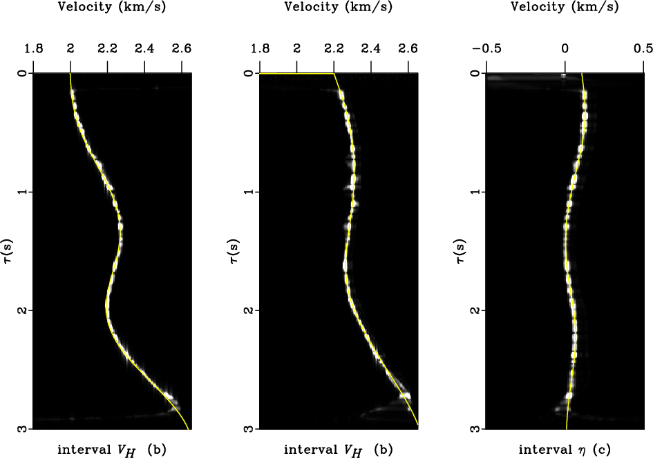
Now, given the slope field ![]() and its zero-slope time field
and its zero-slope time field ![]() , we retrieve interval parameters using equations
27 and 28. In Figure 8, the
estimated NMO (a) horizontal velocities (b) and the anellipticity (c)
parameter are mapped to the appropriate zero-slope time using the
painted zero-slope time
, we retrieve interval parameters using equations
27 and 28. In Figure 8, the
estimated NMO (a) horizontal velocities (b) and the anellipticity (c)
parameter are mapped to the appropriate zero-slope time using the
painted zero-slope time ![]() field (Figure 7c).
The exact interval profiles (yellow lines) are recovered nearly
perfectly although the resolution slightly worsens with respect to the
effective profiles (Figure 6). The main reason is the instability
of the additional numerical differentiation along the
field (Figure 7c).
The exact interval profiles (yellow lines) are recovered nearly
perfectly although the resolution slightly worsens with respect to the
effective profiles (Figure 6). The main reason is the instability
of the additional numerical differentiation along the ![]() direction that all the approaches require.
direction that all the approaches require.
|
|---|
|
intPmasksynth
Figure 7. Fowler's equation based inversion to interval normal moveout (a) horizontal velocity (b) and anellipticity parameter |
|
|
|
|
|
|
Velocity-independent |