|
|
|
|
Time-frequency analysis of seismic data using local attributes |
Seismic instantaneous frequency is the derivative of the instantaneous
phase
Average frequency can be estimated from the time-frequency
map (Cohen, 1989; Steeghs and Drijkoningen, 2001; Sinha et al., 2009; Hlawatsch and Boudreaux-Bartels, 1992; Claasen and Mecklenbräuker, 1980).
Average frequency at a given time is
where ![]() is the time-frequency map. Average frequency measured
by equation 13 is the first moment along the frequency axis of
a time-frequency power spectrum. Saha (1987) and Brian et al. (1993)
analyzed the relationship between instantaneous frequency
and the time-frequency map in detail. Extraction of the attributes
from the time-frequency map of the seismic trace leads to considerable
improvement of the signal-to-noise ratio of the attributes
(Steeghs and Drijkoningen, 2001). We therefore propose applying
equation 13 to our time-frequency map to compute the time-varying
average frequency.
is the time-frequency map. Average frequency measured
by equation 13 is the first moment along the frequency axis of
a time-frequency power spectrum. Saha (1987) and Brian et al. (1993)
analyzed the relationship between instantaneous frequency
and the time-frequency map in detail. Extraction of the attributes
from the time-frequency map of the seismic trace leads to considerable
improvement of the signal-to-noise ratio of the attributes
(Steeghs and Drijkoningen, 2001). We therefore propose applying
equation 13 to our time-frequency map to compute the time-varying
average frequency.
|
|---|
|
ref-6,s-6
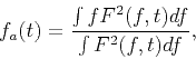
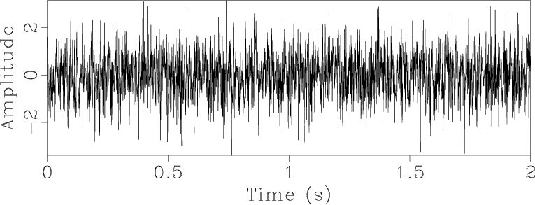
Figure 3. (a) Random reflectivity series. (b) Synthetic seismic trace. |
|
|
|
|---|
|
spec,st-6,proj-6
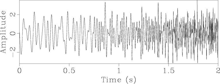
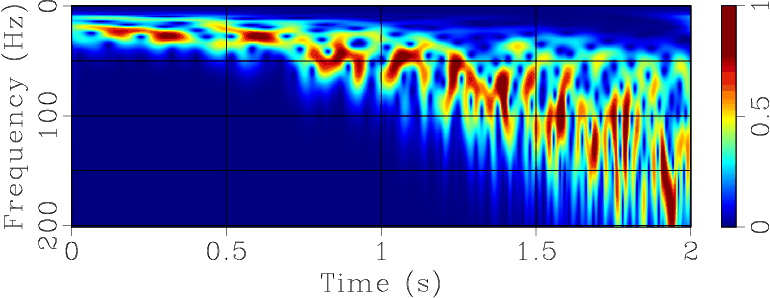
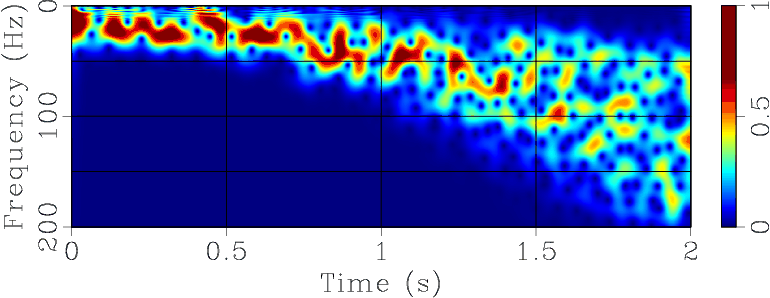
Figure 4. (a) Theoretical time-frequency map, which is scaled by a maximum in the frequency axis. White and black lines indicate dominant frequency and average frequency of Ricker wavelet, respectively. (b) Time-frequency map of the S-transform. (c) Time-frequency map of the proposed method. |
|
|
|
|---|
|
lcf-6
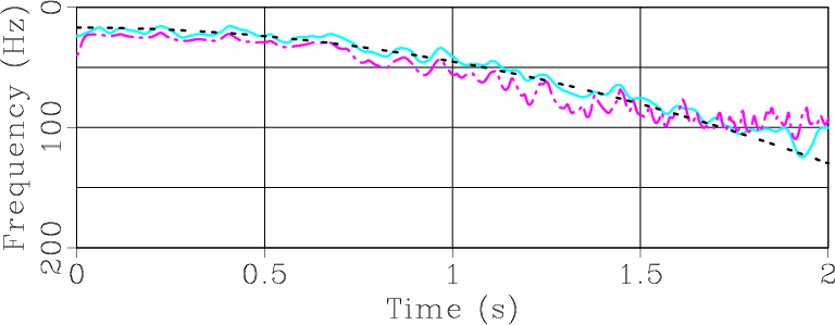
Figure 5. Time-varying average-frequency estimation (blue solid curve: estimated by our method; pink dashed curve: estimated by S-transform; black dot-dashed curve: theoretical curve, which is denoted by black line in Figure 9). |
|
|
We used a synthetic nonstationary seismic trace to illustrate our
approach to estimating time-varying average frequency. Figure 3(b)
shows a synthetic seismic trace generated by nonstationary convolution
(Margrave, 1998) of a random reflectivity series (Figure 3(a))
using a Ricker wavelet, the dominant frequency of which is a function
of time,
![]() . Figure 9 shows the scaled spectrum
of the Ricker wavelet. Both the dominant frequency (white line in
Figure 9 and the bandwidth increase with time. We computed the
average frequency (black line in Figure 9 using equation 13 from
the scaled spectrum of Ricker wavelets. We note that average
frequency is larger than the dominant frequency at high frequencies
for Ricker wavelets.
. Figure 9 shows the scaled spectrum
of the Ricker wavelet. Both the dominant frequency (white line in
Figure 9 and the bandwidth increase with time. We computed the
average frequency (black line in Figure 9 using equation 13 from
the scaled spectrum of Ricker wavelets. We note that average
frequency is larger than the dominant frequency at high frequencies
for Ricker wavelets.
We generated the time-frequency map of the synthetic nonstationary seismic trace using the S-transform (Figure 4(b)) and the proposed method with a 10-point smoothing radius (Figure 4(c)). We observe that the time-frequency map by the proposed method has a bandwidth more similar to that of the time-frequency map of the Ricker wavelet (Figure 9), especially at the high frequencies. We estimated time-varying average frequency curves from the time-frequency map by the proposed method (blue solid curve in Figure 5) and S-transform (pink dashed curve in Figure 5), respectively. Compared with the theoretical curve (black dashed curve in Figure 5), which was computed using equation 13 on the scaled spectrum of Ricker wavelets (Figure 9), the time-varying average frequency estimated by the proposed method is closer to the theoretical one.
|
|
|
|
Time-frequency analysis of seismic data using local attributes |