Shaping regularization in geophysical estimation problems

Smoothing by regularization

Let us consider an application of Tikhonov's regularization to one of the simplest possible estimation problems: smoothing. The task of smoothing is to find a model $\mathbf{m}$ that fits the observed data $\mathbf{d}$ but is in a certain sense smoother. In this case, the forward operator $\mathbf{L}$ is simply the identity operator, and the formal solutions 1 and 3 take the form

$$\widehat{\mathbf{m}} = \left(\mathbf{I} + \epsilon^2\,\m... ...thbf{C} + \epsilon^2\,\mathbf{I}\right)^{-1}\,\mathbf{d}\;.$$ (5)

Smoothness is controlled by the choice of the regularization operator $\mathbf {D}$ and the scaling parameter $\epsilon$.

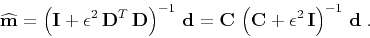
Figure 1 shows the impulse response of the regularized smoothing operator in the 1-D case when $\mathbf {D}$ is the first difference operator. The impulse response has exponentially decaying tails. Repeated application of smoothing in this case is equivalent to applying an implicit Euler finite-difference scheme to the solution of the diffusion equation

$${\frac{\partial \mathbf{m}}{\partial t}} = -\mathbf{D}^T\,\mathbf{D}\,\mathbf{m}$$ (6)

The impulse response converges to a Gaussian bell-shape curve in the physical domain, while its spectrum converges to a Gaussian in the frequency domain.

exp
Figure 1. Left: impulse response of regularized smoothing. Repeated smoothing converges to a Gaussian bell shape. Right: frequency spectrum of regularized smoothing. The spectrum also converges to a Gaussian.

As far as the smoothing problem is concerned, there are better ways to smooth signals than applying equation 5. One example is triangle smoothing (Claerbout, 1992). To define triangle smoothing of one-dimensional signals, start with box smoothing, which, in the $Z$-transform notation, is a convolution with the filter

$$B_k(Z) = \frac{1}{k}\,\left(1 + Z + Z^2 + \cdots + Z^k\right) = \frac{1}{k}\,\frac{1-Z^{k+1}}{1-Z}\;,$$ (7)

where $k$ is the filter length. Form a triangle smoother by correlation of two boxes

$$T_k(Z) = B_k(1/Z)\,B_k(Z)$$ (8)

Triangle smoothing is more efficient than regularized smoothing, because it requires twice less floating point multiplications. It also provides smoother results while having a compactly supported impulse response (Figure 2). Repeated application of triangle smoothing also makes the impulse response converge to a Gaussian shape but at a significantly faster rate. One can also implement smoothing by Gaussian filtering in the frequency domain or by applying other types of bandpass filters.

tri
Figure 2. Left: impulse response of triangle smoothing. Repeated smoothing converges to a Gaussian bell shape. Right: frequency spectrum of triangle smoothing. Convergence to a Gaussian is faster than in the case of regularized smoothing. Compare to Figure 1.

Shaping regularization in geophysical estimation problems