 |
 |
 |
 | Shaping regularization in geophysical estimation problems |  |
![[pdf]](icons/pdf.png) |
Next: Smoothing by regularization
Up: Fomel: Shaping regularization
Previous: Introduction
If the data are represented by vector  , model parameters by
vector
, model parameters by
vector  , and their functional relationship is defined by the
forward modeling operator
, and their functional relationship is defined by the
forward modeling operator  , the least-squares optimization
approach amounts to minimizing the least-squares norm of the residual
difference
, the least-squares optimization
approach amounts to minimizing the least-squares norm of the residual
difference
 . In Tikhonov's regularization approach, one
additionally attempts to minimize the norm of
. In Tikhonov's regularization approach, one
additionally attempts to minimize the norm of  , where
  is the regularization operator. Thus, we are looking for the model
that minimizes the least-squares norm of the compound vector
is the regularization operator. Thus, we are looking for the model
that minimizes the least-squares norm of the compound vector
![$\left[\begin{array}{cc} \mathbf{L m - d} & \epsilon \mathbf{D m}
\end{array}\right]^T$](img10.png) ,
where
,
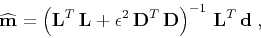
where  is a scalar scaling parameter. The formal solution has the
well-known form
is a scalar scaling parameter. The formal solution has the
well-known form
 |
(1) |
where
 denotes the least-squares estimate of ,
and
denotes the least-squares estimate of ,
and  denotes the adjoint operator. One can carry out the
optimization iteratively with the help of the conjugate-gradient method
(Hestenes and Steifel, 1952) or its analogs. Iterative methods have computational
advantages in large-scale problems when forward and adjoint operators are
represented by sparse matrices and can be computed efficiently
(Saad, 2003; van der Vorst, 2003).
denotes the adjoint operator. One can carry out the
optimization iteratively with the help of the conjugate-gradient method
(Hestenes and Steifel, 1952) or its analogs. Iterative methods have computational
advantages in large-scale problems when forward and adjoint operators are
represented by sparse matrices and can be computed efficiently
(Saad, 2003; van der Vorst, 2003).
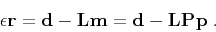
In an alternative approach, one obtains the regularized estimate by
minimizing the least-squares norm of the compound vector
![$\left[\begin{array}{cc} \mathbf{p} & \mathbf{r} \end{array}\right]^T$](img15.png) under the constraint
under the constraint
 |
(2) |
Here  is the model reparameterization operator that
translates vector
is the model reparameterization operator that
translates vector  into the model vector ,
 is the scaled residual vector, and has the
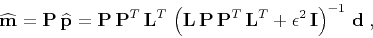
same meaning as before. The formal solution of the preconditioned
problem is given by
is the scaled residual vector, and has the
same meaning as before. The formal solution of the preconditioned
problem is given by
 |
(3) |
where  is the identity operator in the data space.
Estimate 3 is mathematically equivalent to
estimate 1 if
is the identity operator in the data space.
Estimate 3 is mathematically equivalent to
estimate 1 if
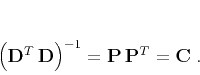
 is invertible
and
is invertible
and
 |
(4) |
Statistical theory of least-squares estimation connects  with the model covariance operator (Tarantola, 2004). In a more
general case of reparameterization, the size of may be
different from the size of , and may not have
the full rank. In iterative methods, the preconditioned formulation
often leads to faster convergence. Fomel and Claerbout (2003) suggest
constructing preconditioning operators in multi-dimensional problems
by recursive helical filtering.
with the model covariance operator (Tarantola, 2004). In a more
general case of reparameterization, the size of may be
different from the size of , and may not have
the full rank. In iterative methods, the preconditioned formulation
often leads to faster convergence. Fomel and Claerbout (2003) suggest
constructing preconditioning operators in multi-dimensional problems
by recursive helical filtering.
|
|
|
|
| Shaping regularization in geophysical estimation problems | |
|
Next: Smoothing by regularization
Up: Fomel: Shaping regularization
Previous: Introduction
2013-03-02