|
|
|
|
OC-seislet: seislet transform construction with differential offset continuation |
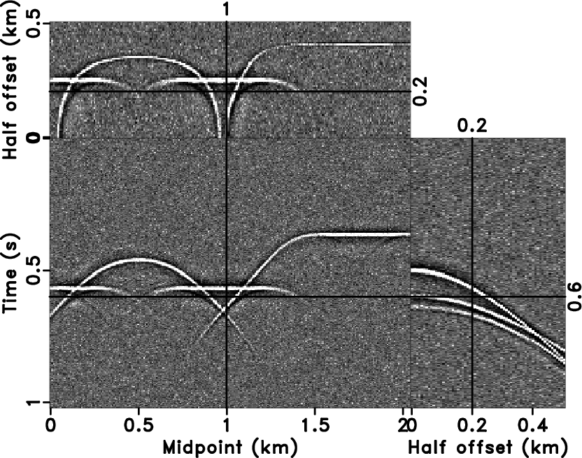
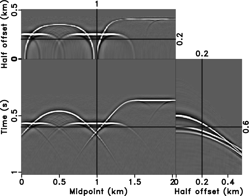
We continue to use the synthetic model from Figure 1 to
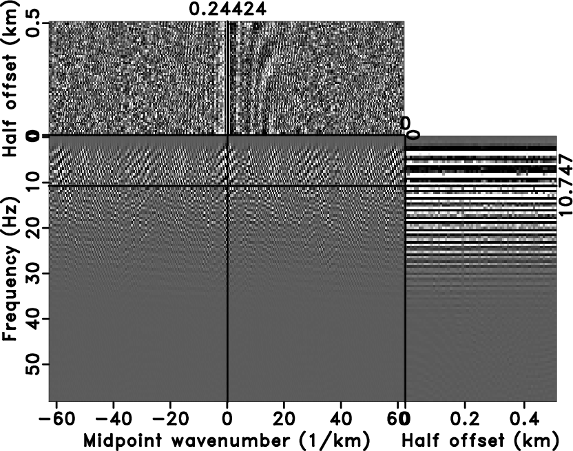
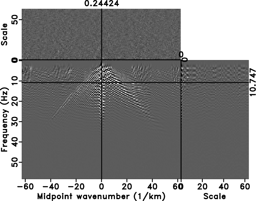
test the proposed method. Figure 6 is the data with
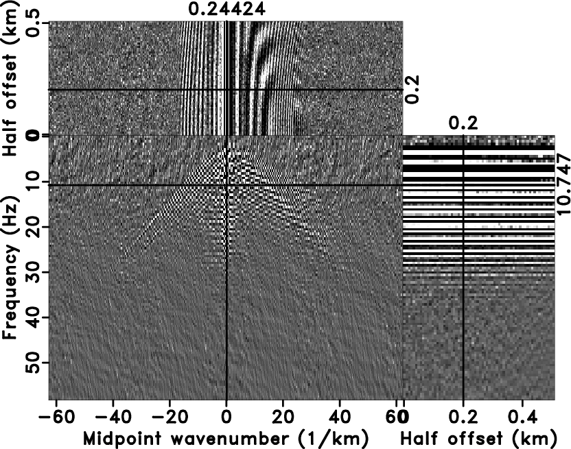
normally-distributed random noise added. Figure 7a
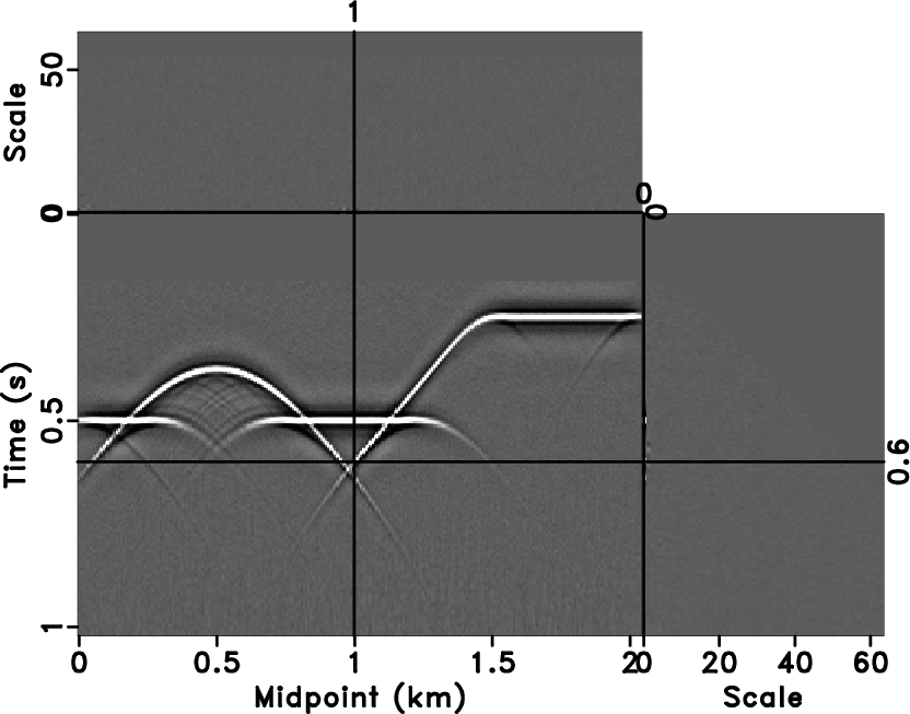
shows the datacube in the ![]() -
-![]() -offset domain after the
log-stretched NMO correction and a double Fourier transform along the
stretched time axis and midpoint axis. We run the OC-seislet
transform in parallel on individual frequency
slices. Figure 7b shows the OC-seislet
coefficients. All reflection information is concentrated in a small
scale range. However, since random noise cannot be predicted well by
the offset-continuation operator, it spreads throughout the whole
transform domain. The inverse Fourier transform both in time and
midpoint directions and the inverse log-stretch return the OC-seislet
coefficients to the time-midpoint-scale domain. The coefficients at
the zero scale represent stacking along the offset direction, which
is equivalent to the DMO stack (Figure 8b).
-offset domain after the
log-stretched NMO correction and a double Fourier transform along the
stretched time axis and midpoint axis. We run the OC-seislet
transform in parallel on individual frequency
slices. Figure 7b shows the OC-seislet
coefficients. All reflection information is concentrated in a small
scale range. However, since random noise cannot be predicted well by
the offset-continuation operator, it spreads throughout the whole
transform domain. The inverse Fourier transform both in time and
midpoint directions and the inverse log-stretch return the OC-seislet
coefficients to the time-midpoint-scale domain. The coefficients at
the zero scale represent stacking along the offset direction, which
is equivalent to the DMO stack (Figure 8b).
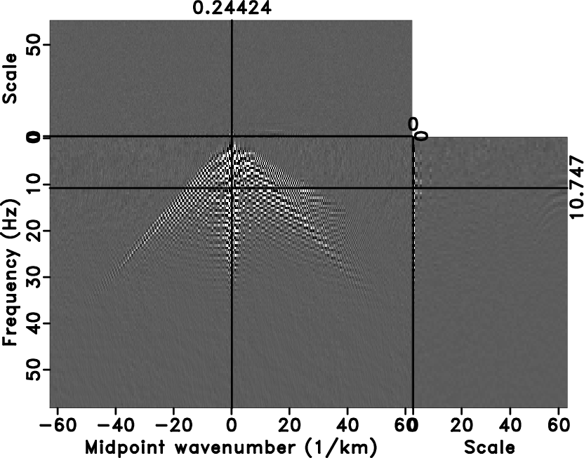
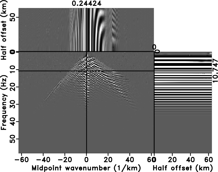
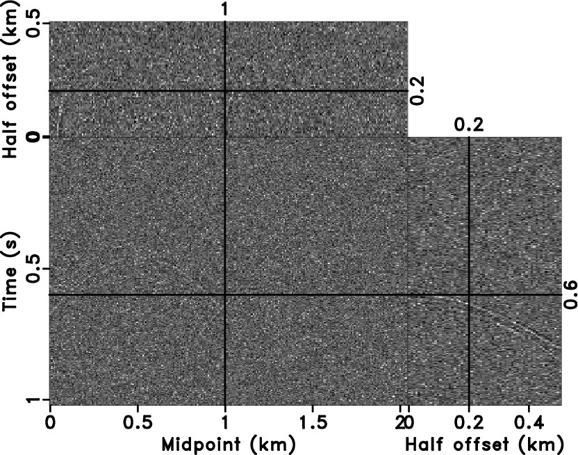
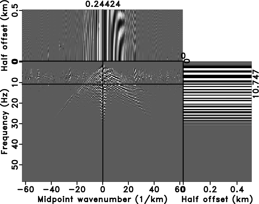
We use a soft-thresholding method to separate reflection and random
noise in the OC-seislet domain. Figure 8a
displays the result after the inverse OC-seislet transform. Compared
with Figure 7a, data in the ![]() -
-![]() -offset domain
contain only useful information. Figure 9b shows
the denoising result in the
-offset domain
contain only useful information. Figure 9b shows
the denoising result in the ![]() -
-![]() -offset domain after the double
inverse Fourier transform, the inverse log-stretch and the inverse
NMO. All characteristics of reflection and diffraction events are
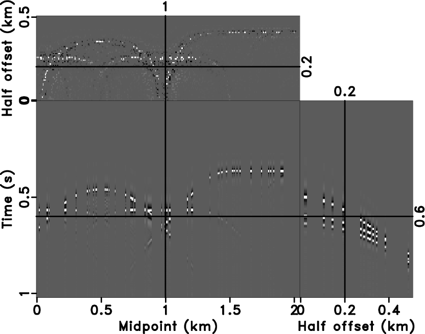
preserved well. For comparison, we used PWD-seislet transform and
soft-thresholding method with the same threshold values to process
the noisy data (Figure 6). The result is shown in
Figure 9a. Because PWD-seislet transform is based
on the local dip information, a mixture of different dips from the
triplications makes it difficult to process the data in individual
common-midpoint gathers. The PWD-seislet transform compresses all
information along the local events slopes in each common-midpoint
gather. It separates reflection signal and noise but smears the
crossing events, especially at the far offset. The corresponding
signal-to-noise ratios for denoised results with PWD-seislet
transform and OC-seislet transform are 24.95 dB and 41.45 dB,
respectively. The differences (Figure 10) between
noisy data (Figure 6) and denoised results with
PWD-seislet transform (Figure 9a) and OC-seislet
transform (Figure 9b) further
illustrate the effectiveness of the OC-seislet
transform.
-offset domain after the double
inverse Fourier transform, the inverse log-stretch and the inverse
NMO. All characteristics of reflection and diffraction events are
preserved well. For comparison, we used PWD-seislet transform and
soft-thresholding method with the same threshold values to process
the noisy data (Figure 6). The result is shown in
Figure 9a. Because PWD-seislet transform is based
on the local dip information, a mixture of different dips from the
triplications makes it difficult to process the data in individual
common-midpoint gathers. The PWD-seislet transform compresses all
information along the local events slopes in each common-midpoint
gather. It separates reflection signal and noise but smears the
crossing events, especially at the far offset. The corresponding
signal-to-noise ratios for denoised results with PWD-seislet
transform and OC-seislet transform are 24.95 dB and 41.45 dB,
respectively. The differences (Figure 10) between
noisy data (Figure 6) and denoised results with
PWD-seislet transform (Figure 9a) and OC-seislet
transform (Figure 9b) further
illustrate the effectiveness of the OC-seislet
transform.
|
|---|
|
noise
Figure 6. 2-D noisy data in |
|
|
|
|---|
|
input,tran
Figure 7. Noisy data in |
|
|
|
|---|
|
ithr,inv-tran
Figure 8. Thresholded data in |
|
|

|
|---|
|
nidwt,inver
Figure 9. Denoised result by different methods. PWD-seislet transform (a) and OC-seislet transform (b). (Compare with Figure 2.) |
|
|

|
|---|
|
diff1,diff2
Figure 10. Difference between noisy data (Figure 6) and denoised results with different methods (Figure 9). PWD-seislet transform (a) and OC-seislet transform (b). |
|
|
For a data regularization test, we remove 80% of randomly selected traces (Figure 11a) from the ideal data (Figures 2a). The complex dip information makes it extremely difficult to interpolate the data in individual common-offset gathers. The dataset is also non-stationary in the offset direction. Therefore, a simple offset interpolation scheme would also fail. Figure 11b shows the data after NMO correction, log-stretch transform, and double Fourier transforms. The missing traces introduce spatial artifacts in midpoint-wavenumber axis and discontinuities along the offset direction. After the OC-seislet transform, the reflection information can be predicted and compressed. Meanwhile, the artifacts spread over the whole transform domain (Figure 12a). The simple soft-thresholding algorithm (i.e., the iterative strategy with only one iteration) removes most of the artifacts, and the inverse OC-seislet transform reconstructs the major reflection information according to the offset-continuation prediction (Figure 12b).
|
|---|
|
czero,cinput
Figure 11. Synthetic data with 80% traces removed (a) and missing data in |
|
|
|
|---|
|
ctran,cithr
Figure 12. OC-seislet coefficients in |
|
|
2four3pocs,cpocswidth=0.7 Interpolated results using iterative thresholding with different sparse transforms. 3-D Fourier transform (a) and OC-seislet transform (b). (Compare with Figure 2)
One can also employ an iterative soft-thresholding strategy to implement missing data interpolation. This method recovers missing traces as long as seismic data are sparse enough in the transform domain. To demonstrate the superior sparseness of the OC-seislet coefficients, we compare the proposed method with the 3-D Fourier transform. Figure 13a displays the interpolated result after a 3-D Fourier interpolation using iterative thresholding (Abma and Kabir, 2006). The Fourier transform cannot provide enough sparseness of coefficients for complex reflections and, therefore, fails in recovering all missing traces. The OC-seislet transform is based on a physical prediction, and provides a much sparser domain for both reflections and diffractions. Iterative thresholding succeeds in interpolating the missing traces (Figure 13b).
|
|
|
|
OC-seislet: seislet transform construction with differential offset continuation |