3D velocity-independent elliptically-anisotropic moveout correction

Examples

cmp3d,nmo063d
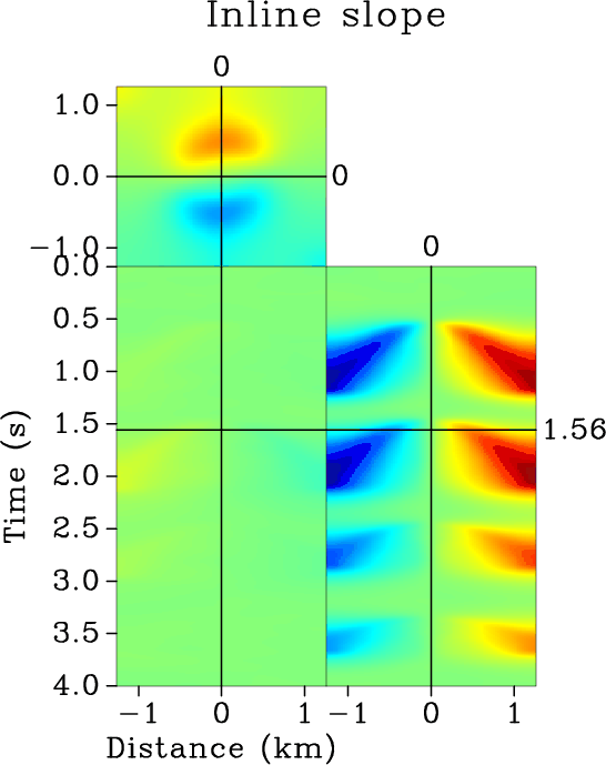
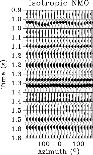
Figure 2. (a.) A synthetic 3D CMP gather with four events of varying apparent elliptical anisotropy. The three panels in the display show a time-slice view (upper square panel), a crossline view (central panel), and an inline view (right panel) of the same volume. (b.) An isotropic NMO correction using a picked velocity function appropriate for flattening certain events. At best, isotropic NMO can flatten either the inline or crossline directions well, but there is no single velocity function that will flatten both.

pxsmooth3d,pysmooth3d,PNMO3d
Figure 3. The (a.) inline and (b.) crossline slopes of the CMP gather from Figure 2(a). (c.) These slopes are used with equation 8 to automatically perform the proposed elliptically anisotropic moveout correction. All four events are flattened perfectly where the slopes are not aliased.

We provide two examples to illustrate the performance of our approach. In the first example, we consider a simple 3D synthetic CMP gather (Figure 2(a)) with four events, each with a different degree of apparent azimuthal anisotropy. The synthetic CMP in Figure 2(a) was created by first specifying the moveout slowness matrix, $\tensor{W}$ for each event. Each of the four events was modeled individually by applying inverse 3D NMO to a flat reflection based on equation 1. The exact parameters used to model the four events are specified in Table 1. The four events were then added together into a single CMP gather with a small amount of random noise (10% of the signal amplitude). The result of this approach differs from real cases in that the traveltime surface for each of the events is completely independent from overlying events. However, this approach allows us to specify the exact moveout slownesses of each the events without additional work.

Event Moveout Parameters
Event	$t_0$ (s)	$W_x (s^2/km^2)$	$W_y (s^2/km^2)$	$W_{xy} (s^2/km^2)$	$\alpha (^\circ )$
A	0.59	0.14	0.16	-0.01	14.0
B	1.53	0.30	0.30	-0.04	-44.3
C	2.51	0.32	0.26	-0.03	-21.8
D	3.41	0.24	0.25	-0.005	26.57

Table 1. Moveout parameters used for events in Figure 2(a).

Conventional velocity semblance scans may yield multiple peaks for the same event when apparent azimuthal anisotropy is present. One must interpret the correct velocity in these areas, which can lead to inconsistent results between different processing geophysicists, since the cause of multiple semblance panel peaks can be ambiguous (multiples, noise, anisotropy, etc.). Resolving this ambiguity properly can add even more time and work to the production approach. Figure 2(b) shows a possible result of picking a single velocity profile which flattens certain events in either the inline or crossline view. For a root-mean-square velocity model, if an intermediate value is chosen for each event, both directions are flattened poorly. Event B has a particularly difficult scenario for the production approach; the symmetry axes are nearly 45$^\circ$ from the acquisition axes, which makes the apparent moveout velocities along the x and y axes practically equal. A production velocity analysis is likely to not even detect the anisotropy in this case, because viewed from the acquisition axes, event B appears isotropic. The time-slice panel of Figure 2(b) reveals the poor performance of the isotropic NMO correction along other source-receiver azimuths of event B.

By measuring the local slopes of an input CMP gather as a volumetric attribute, the geometry of each traveltime surface is captured, even away from the x and y acquisition axes. Figures 3(a) and 3(b) show sections of the automatically measured inline and crossline slope volumes for the CMP from Figure 2(a). The time-slice views clarify that the slopes are measured in the x and y directions throughout the volume, not just along the x and y zero-offset axes. Comparison of the slope volumes with Figure 2(a) also shows that there are clearly non-zero slopes in areas without data. No initial slope fields were used to get these measurements, but the results of the plane-wave destruction filter application were regularized with a smoothing constraint by using shaping regularization (Fomel, 2007). This constraint is enforced to help ensure that the moveout correction varies both spatially and temporally in a stable fashion. In Figure 3(c), the velocity-independent elliptically anisotropic moveout correction is applied using these slopes, and all of the events are flattened well in both directions. The time-slice view of Figure 3(c) now shows the overall superior performance of the velocity-independent correction, but also reveals its limitations. As events become steep relative to the trace spacing, local slope measurements can be aliased. Towards the corners of the example gather, the slopes become too steep to be measured reliably, and in these areas, the automatic moveout correction performs poorly. In field data, crossline trace spacing is often much coarser than inline spacing, which may lead to similar aliasing problems. However, the effects of aliasing can often be mitigated with a few simple extra steps. By first applying a constant velocity isotropic NMO correction to the data before measuring slopes, the events will be flatter and less likely to have aliased slopes at far offsets. An inverse NMO correction using the constant velocity can then be applied to the measured slopes. The constant velocity can then be converted to $p_x$ and $p_y$ components and added to the slope measurements to obtain the unaliased slope fields of the input CMP gather.

Another perspective of the same test is shown in Figures 4(a) and 4(b). The traces from the synthetic CMP gather have been binned into offset and azimuth coordinates to display the familiar sinusoidal signature of azimuthal traveltime variations. The various squared traveltime shifts ($t_\Delta$ values) applied by the automatic NMO correction were computed during implementation using equation 8, and then stored as a volumetric attribute. For each of the events, time-slices of this volume are shown in Figures 5(a)-5(d). The elliptical variation is clearly displayed for events A, B, and C, but the subtle variation for event D makes it difficult to detect the apparent anisotropy. Each time-slice from the same volume was re-indexed into a vector following the scheme described in the previous section, and then fed into a least-squares solver for equation 15 to yield $\tensor{W}(t_0)$ . The results of this inversion are displayed in Figures 6(a)-6(b). At the times of the events, all three parameters have been extracted accurately. The shaping regularization used to create smooth slope fields also leads to similar smoothness in the $\tensor{W}$ estimates. Because of the random noise in the synthetic data, slope measurements away from events are also random. The best-fit surface through these random slopes tends to be a flat plane, which is characterized on a CMP gather by zero slowness, causing the $W_x$ and $W_y$ estimates to tend toward zero between events. It is important to note that the values shown in Figures 6(a)-6(d) each rely on the accuracy of the NMO shifts computed at the corresponding value of $t_0$ . Only the sparse times of this synthetic CMP gather with data have meaningful slope estimates and therefore meaningful $\tensor{W}$ and $\alpha$ estimates.

oacmp,oaPNMO
Figure 4. (a.) A common offset (0.75 km) display of CMP from Figure 2(a) with azimuth on the horizontal axis. (b.) The same traces after the automatic moveout correction. All events are shifted up to their appropriate $t_0$ and flattened.

deltaTslice1,deltaTslice2,deltaTslice3,deltaTslice4
Figure 5. Traveltime squared shifts ( $t_{\Delta }(t_0,x,y)$ ) for each event. (a.) Event A. (b.) Event B. (c.) Event C. (d.) Event D.

The extracted moveout slowness matrices $\tensor{W}(t_0)$ are used with equation 2 to estimate $\alpha (t_0)$ . The results of estimating $\alpha (t_0)$ are displayed in Figure 6(d), and the values at the times of each event are accurate. We conclude this example by solving for NMO slowness-squared as using $\alpha (t_0)$ and the corresponding eigenvalues at each $t_0$ with equation 5. These results, shown in Figures 7(a)-7(d) show that for all four events, the angle of anisotropy is detected. From this volume, the principal moveout directions are readily determined, the fast and slow axes are resolved, and the apparent anisotropy (the ratio or difference of $V_{fast}$ and $V_{slow}$ ) is measurable.

Wxinv,Wyinv,Wxyinv,InvAlpha
Figure 6. Elements of $\tensor{W}(t_0)$ inverted from $t_{\Delta }(t_0,x,y)$ surfaces: (a.) $W_x$ . (b.) $W_y$ . (c.) $W_{xy}$ . (d.) Azimuth angle $\alpha (t_0)$ computed from $\tensor{W}(t_0)$ .

slowsqrdslice1,slowsqrdslice2,slowsqrdslice3,slowsqrdslice4
Figure 7. Time-slice views of NMO slowness-squared values computed for each event.(a.) Event A. (b.) Event B. (c.) Event C. (d.) Event D.

supercube
Figure 8. 3D view of a supergather from the McElroy data set, West Texas, US. Although the data has been isotropically NMO corrected, the time-slice view shows a subtle directional trend to the flatness of an event at 0.978 s.

super21-anisow,pmag3-anisow,pnmo-oa2-anisow
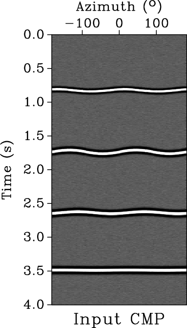
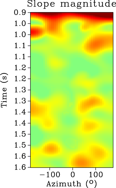
Figure 9. A time-versus-azimuth panel of traces for a range of offsets from 3.6-4.0 km from the McElroy data set. The central panel shows local slope magnitudes corresponding to the left input panel. The slope magnitude was computed as $\sqrt {p_x^2+p_y^2}$ . The same data after an automatic moveout correction has been applied as a residual moveout correction is shown on the right.

We next demonstrate a potential application of the automatic moveout correction on a real data example. In this case, we apply the automatic elliptically anisotropic moveout correction as a residual moveout correction. A subset of the McElroy data set from West Texas was formed into a supergather seen in Figure 8. Figure  shows a common offset (3.6-4.0 km) time-versus-azimuth display of the same data, where azimuthal anisotropy is evident for several events. In Figure , the magnitude of the local slope is shown for the initial data. The areas with higher slope values highlight areas that were not ideally flattened by the prior isotropic NMO correction. The region of the highest slopes along the top of the figure is due to the proximity of the prior NMO mute at about 0.8 $s$ . Figure  shows the results of applying two iterations of the proposed moveout correction. Further iterations will continue to flatten later events as distortions from overlying layers are removed. The events in the results are already noticeably flatter, and will therefore produce a cleaner stack.

3D velocity-independent elliptically-anisotropic moveout correction