|
|
|
|
3D velocity-independent elliptically-anisotropic moveout correction |
where ![]() is the event arrival time,
is the event arrival time, ![]() is the moveout corrected time, and
is the moveout corrected time, and ![]() and
and ![]() are the components of full offset in the x and y survey directions, respectively.
are the components of full offset in the x and y survey directions, respectively. ![]() and
and ![]() are the conventionally-measured moveout slownesses squared values (along the same survey coordinates). Equation 1 describes NMO with elliptical velocity, where the third parameter,
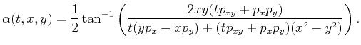
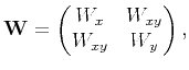
are the conventionally-measured moveout slownesses squared values (along the same survey coordinates). Equation 1 describes NMO with elliptical velocity, where the third parameter, ![]() , arises from observing the ellipse from rotated coordinates. In practice, one can perform elliptically anisotropic NMO using conventional velocity picking in the inline and crossline directions, but the principal directions of moveout must also be estimated. Rewriting equation 1 as a matrix-vector multiplication between the offset vector and the slowness matrix
, arises from observing the ellipse from rotated coordinates. In practice, one can perform elliptically anisotropic NMO using conventional velocity picking in the inline and crossline directions, but the principal directions of moveout must also be estimated. Rewriting equation 1 as a matrix-vector multiplication between the offset vector and the slowness matrix
![]() allows one to solve for the angle between the acquisition coordinates and the medium symmetry axes, denoted as
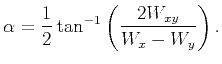
allows one to solve for the angle between the acquisition coordinates and the medium symmetry axes, denoted as ![]() here. This can be done either by finding the eigenvectors of the system (Grechka and Tsvankin, 1998), or by using geometric arguments and well-known relations between the formulas for a rotated ellipse and its unrotated equivalent (Weisstein, 2009). Using the latter approach gives an expression for
here. This can be done either by finding the eigenvectors of the system (Grechka and Tsvankin, 1998), or by using geometric arguments and well-known relations between the formulas for a rotated ellipse and its unrotated equivalent (Weisstein, 2009). Using the latter approach gives an expression for ![]() in terms of conventional slowness parameters,
in terms of conventional slowness parameters,

|
|---|
|
HTINMO
Figure 1. Elliptic NMO velocity depends on the natural symmetry axes (a-b), not the acquisition coordinates (x-y). The angle |
|
|
In this expression, ![]() is the angle from a survey axis measured counter-clockwise toward the nearest symmetry axis. If
is the angle from a survey axis measured counter-clockwise toward the nearest symmetry axis. If ![]() is equal to
is equal to ![]() , then the arc-tangent argument goes to infinity, corresponding to
, then the arc-tangent argument goes to infinity, corresponding to
![]() . Although equation 2 is a straightforward way of finding the coordinate rotation angle, finding the eigenvalues and eigenvectors allows one to resolve between the fast and slow principal moveout directions. The eigenvalues
. Although equation 2 is a straightforward way of finding the coordinate rotation angle, finding the eigenvalues and eigenvectors allows one to resolve between the fast and slow principal moveout directions. The eigenvalues
![]() and
and
![]() of the slowness matrix,
of the slowness matrix,
can be found following Grechka and Tsvankin (1998). Rewritten here in our notation, they demonstrate how the eigenvalues,
can be used together with ![]() to solve for the NMO slowness
to solve for the NMO slowness ![]() as a function of source-receiver azimuth
as a function of source-receiver azimuth ![]() :
:
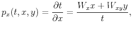
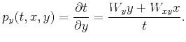
Since equation 1 describes the predicted hyperbolic traveltime curve on a CMP gather for a variety of cases where either real or apparent elliptical anisotropy may be present, the local slope of an event on an inline or crossline CMP gather can be related to the conventional moveout slowness parameters by taking the derivative of 1 with respect to ![]() and
and ![]() . Ignoring higher order terms and assuming the parameters vary slowly along
. Ignoring higher order terms and assuming the parameters vary slowly along ![]() and
and ![]() , gives a first-order approximation of how the measured slopes relate to conventional moveout parameters:
, gives a first-order approximation of how the measured slopes relate to conventional moveout parameters:
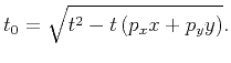
By substitution back into 1, we arrive at the velocity-independent expression for 3D elliptical moveout in terms of local slopes:
Notice that only two parameters (![]() and
and ![]() ) must be measured to completely predict the NMO corrected time. More importantly, these parameters can be measured automatically using a local slope estimation algorithm, such as plane-wave destruction (Fomel, 2002). Equation 8 is a 3D extension for the 2D equation from Ottolini (1983).
) must be measured to completely predict the NMO corrected time. More importantly, these parameters can be measured automatically using a local slope estimation algorithm, such as plane-wave destruction (Fomel, 2002). Equation 8 is a 3D extension for the 2D equation from Ottolini (1983).
Automated processes allow one to save time spent on a project, but it may seem that the insight and information gained during a more interactive conventional processing flow would be lost. A significant part of production velocity analysis involves picking or examining the velocity model directly, which provides an early and intuitive link between the seismic data and the subsurface geology. The velocity model and anisotropy information are themselves invaluable sources of geologic information. They also control the positioning of events in the final image, so an ability to extract these parameters is desirable.
The relation between local slopes and moveout velocity has been documented for the 2D case (Wolf et al., 2004; Ottolini, 1983; Fomel, 2007). In the 3D case where apparent azimuthal anisotropy is present, at least three conventional slowness or velocity-like values are needed to characterize moveout (![]() ,
, ![]() , and
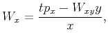
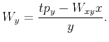
, and ![]() from equation 1). Although equation 8 suggests they are not necessary for moveout in terms of local slopes, these values can be used to characterize anisotropy, and may also be useful for other subsequent processing. Simply rearranging equations 6 and 7 gives expressions for
from equation 1). Although equation 8 suggests they are not necessary for moveout in terms of local slopes, these values can be used to characterize anisotropy, and may also be useful for other subsequent processing. Simply rearranging equations 6 and 7 gives expressions for ![]() and
and ![]() :
:
and,
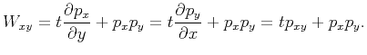
Both of these parameters require an estimate of ![]() . A first-order approximation of
. A first-order approximation of ![]() can be found by differentiating equation 6 with respect to
can be found by differentiating equation 6 with respect to ![]() or equation 7 with respect to
or equation 7 with respect to ![]() :
:
Since slopes are measured as a local attribute, the inline and crossline local slopes comprise data volumes with the same dimensions and coordinates as the input CMP. Applying a 1D derivative filter to these volumes allows one to obtain either mixed-derivative in equation 11, and solve for the apparent anisotropy angle ![]() , using equation 1. This angle can also be expressed in terms of local slopes. Combining equations 9, 10, and 11 yields,
, using equation 1. This angle can also be expressed in terms of local slopes. Combining equations 9, 10, and 11 yields,
Now everything needed to express ![]() independently of velocity is found in equations 11 and 12. Combining them with equation 2 gives,
independently of velocity is found in equations 11 and 12. Combining them with equation 2 gives,
Implementing equation 13 creates an attribute for each input data sample describing the counter-clockwise azimuthal angle between the symmetry coordinates and the acquisition coordinates. Applying NMO to this attribute volume yields
![]() , which should then theoretically be constant at each time-slice if the moveout were exactly described by equation 1.
, which should then theoretically be constant at each time-slice if the moveout were exactly described by equation 1.
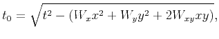
Finding local estimates of slowness and anisotropy parameters using equations 9-13 remains at this point only an interesting theoretical idea. A more robust and practical approach to extracting velocity and anisotropy parameters is to exploit the shear number of volumetric slope measurements made to perform the velocity-independent NMO correction. For a given CMP with dimensions (
![]() ), the NMO correction applies a shift of time-squared,
), the NMO correction applies a shift of time-squared,
which can be automatically computed for every output coordinate using equation (8) and stored as another volume of the same dimensions. Once NMO is applied, the time axis of the CMP gather represents ![]() , so the slowness matrix
, so the slowness matrix
![]() and
and ![]() should each be constant for a given time value. Each time-slice from either the data or one of the attribute volumes can be viewed as an (
should each be constant for a given time value. Each time-slice from either the data or one of the attribute volumes can be viewed as an (
![]() ) matrix, which can be re-indexed into a vector of length (
) matrix, which can be re-indexed into a vector of length (
![]() ). If the x and y indexes from the time-slice are
). If the x and y indexes from the time-slice are ![]() and
and ![]() respectively, then the value from position (
respectively, then the value from position (![]() ) in the matrix is mapped to the
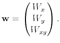
) in the matrix is mapped to the ![]() position in the vector. Using this notation, a highly overdetermined problem follows from writing equation 1 as a matrix-vector multiplication:
position in the vector. Using this notation, a highly overdetermined problem follows from writing equation 1 as a matrix-vector multiplication:
where the ![]() element of
element of
![]() is,
is,
the ![]() row of
row of
![]() is given by the vector,
is given by the vector,
and
Linear system 15 has (
![]() ) equations with only three unknowns. By solving 15 for each time-slice in the output CMP, we construct the slowness matrix
) equations with only three unknowns. By solving 15 for each time-slice in the output CMP, we construct the slowness matrix
![]() , and use it with equations 13, 4, and 5 to extract the coordinate rotation angle
, and use it with equations 13, 4, and 5 to extract the coordinate rotation angle
![]() and the NMO slowness as a function of azimuth,
and the NMO slowness as a function of azimuth,
![]() .
.
|
|
|
|
3D velocity-independent elliptically-anisotropic moveout correction |
![$\displaystyle \lambda _{1,2}=\frac{1}{2}\left[ W_x+W_y\pm \sqrt{(W_x-W_y)^2+4W_{xy}^2}\right],$](img20.png)
![$\displaystyle W_x-W_y=\frac{t}{xy}[yp_x-xp_y+(p_{xy}+(x^2-y^2)\frac{p_xp_y}{t})].$](img32.png)