|
 |
 |
 | Accelerated plane-wave destruction |  |
![[pdf]](icons/pdf.png) |
Next: Bibliography
Up: Chen, Fomel & Lu:
Previous: Acknowledgments
If all the coefficients of  are polynomials of
  ,
equation 4 is also a polynomial of ,
and the plane-wave destruction equation becomes
in turn a polynomial equation of .
The problem is to design a
,
equation 4 is also a polynomial of ,
and the plane-wave destruction equation becomes
in turn a polynomial equation of .
The problem is to design a  points filter
with polynomial coefficients
such that the allpass system
points filter
with polynomial coefficients
such that the allpass system
 can approximate
the phase-shift operator
can approximate
the phase-shift operator
 .
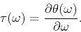
Denoting the phase response of the system as
.
Denoting the phase response of the system as
 ,
that is
,
that is
 ,
the group delay of the system is
,
the group delay of the system is
 |
(24) |
The maximally flat criteria designs a filter
with a smoothest phase response.
There are  unknown coefficients in
  ,
so we can add flat constraints for the first
,
so we can add flat constraints for the first  th order deviratives
of the phase response.
It becomes
(Zhang, 2009, equation 7)
th order deviratives
of the phase response.
It becomes
(Zhang, 2009, equation 7)
 |
(25) |
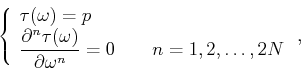
which is equivalent to the following linear maximally flat conditions
(Thiran, 1971):
 |
(26) |
where
 and
and
 is the fractional delay of
  or
or  .
.
In order to solve  from the above equations,
Thiran (1971) used an additional condition
from the above equations,
Thiran (1971) used an additional condition  ,
which leads
,
which leads  to be a fractional function of .
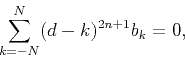
Differently from that, we use the following condition,
to be a fractional function of .
Differently from that, we use the following condition,
 |
(27) |
where can be proved to be polynomials of .
Let vector
![$\mathbf b=[b_0,b_N,\dots,b_1,b_{-1},\dots,b_{-N}]^\textrm T$](img120.png) .
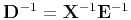
Combining equations I-3 and I-4,
we rewrite them into the following matrix form:
.
Combining equations I-3 and I-4,
we rewrite them into the following matrix form:
The matrix on the left side, denoted as  ,
can be split into four blocks
,
can be split into four blocks
![$\left[\begin{array}{c\vert c}
\tensor A & \tensor B \hline \tensor C & \tensor D
\end{array}\right]$](img123.png) as shown above.
Following the lemma of matrix inversion,
as shown above.
Following the lemma of matrix inversion,
![\begin{displaymath}
\tensor V^{-1}=\left[\begin{array}{cc}
(\tensor A-\tensor B\...
...\tensor C)^{-1}\tensor B\tensor D^{-1} \\
\end{array}\right],
\end{displaymath}](img124.png) |
(28) |
therefore the coefficients
![\begin{displaymath}
\mathbf b=\tensor V^{-1}[1,0,\dots,0]^\textrm T=
\left[\begi...
... A-\tensor B\tensor D^{-1}\tensor C)^{-1}
\end{array}\right].
\end{displaymath}](img125.png) |
(29) |
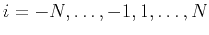
Let subindex
 and
and  .
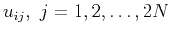
Submatrix
.
Submatrix  can be expressed as
so
 .
Denoting
.
Denoting
 with elements
 ,
as
,
as  is a Vandermonde matrix,
 and Lagrange intepolating polynomials have the following relationship:
 |
(30) |
where
 ,
and
,
and  is the Lagrange polynomial related to the basis
  ,
,
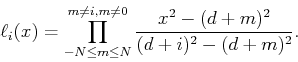 |
(31) |
Substituting the above equation, and  into equation I-7,
we can prove equation I-7.
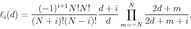
It follows that
into equation I-7,
we can prove equation I-7.
It follows that
![\begin{displaymath}[\tensor E^{-1}\tensor C]_i=d\ell_i(d),
\end{displaymath}](img141.png) |
(32) |
![\begin{displaymath}[\tensor D^{-1}\tensor C]_i=
[\tensor X^{-1}\tensor E^{-1}\tensor C]_i=
\frac{d}{d+i}\ell_i(d),
\end{displaymath}](img142.png) |
(33) |
with
 |
(34) |
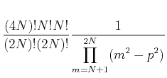
Thus hence
and
![\begin{displaymath}[\tensor A-\tensor B\tensor D^{-1}\tensor C]^{-1} =
\frac{(2N)!(2N)!}{(4N)!N!N!}
\prod_{m=N+1}^{2N}(m^2-p^2).
\end{displaymath}](img147.png) |
(36) |
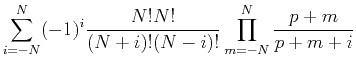
It is the coefficient  , a -th degree polynomial of .
Substituting it into equation I-6,
the coefficients at
, a -th degree polynomial of .
Substituting it into equation I-6,
the coefficients at
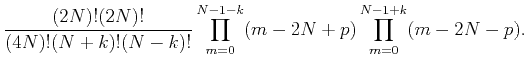
 are expressed as
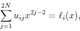
With the additional condition I-4 in points approximation,
all the coefficients are polynomials of of -th degree.
Thus the plane-wave destruction equation 6
therefore is proved to be a polynomial equation of -th degree.
|
|
|
|
| Accelerated plane-wave destruction | |
|
Next: Bibliography
Up: Chen, Fomel & Lu:
Previous: Acknowledgments
2013-03-02
![\begin{displaymath}
\left[\begin{array}{c\vert cccccc}
1 & 1 & \dots & 1 & 1 & \...
...begin{array}{c}
1 0 0 \vdots 0
\end{array}\right].
\end{displaymath}](img121.png)
![\begin{eqnarray*}
\tensor D &=& \tensor E\tensor X \\
&=&
\left[\begin{array}{c...
...} \vdots x_{-1} x_1 \vdots x_N
\end{array}\right],
\end{eqnarray*}](img129.png)