|
 |
 |
 | Fractal heterogeneities in sonic logs
and low-frequency scattering attenuation |  |
![[pdf]](icons/pdf.png) |
Next: Fractal statistics
Up: Browaeys & Fomel: Fractals
Previous: Introduction
Let us consider the spatial fluctuations of seismic velocities to be small and to
constitute a second-order stochastic process.
We describe the fluctuations by using different realizations of the random function  with the expectation value
 and with the spatial covariance
depending on the relative distance
and with the spatial covariance
depending on the relative distance  defined by
where  is the standard deviation and
  is the spatial autocorrelation
function with
is the spatial autocorrelation
function with
 .
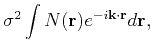
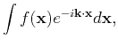
The energy spectrum
.
The energy spectrum
 of the fluctuations in
  dimensions (
 ) is
related to the autocorrelation by the Wiener-Khintchine theorem (Born and Wolf, 1964):
) is
related to the autocorrelation by the Wiener-Khintchine theorem (Born and Wolf, 1964):
where  is the spatial wave vector and
  is the Fourier transform of .
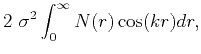
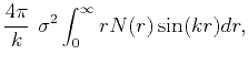
The energy spectrum in equation 2 can be simplified, for an isotropic correlation function, to
is the Fourier transform of .
The energy spectrum in equation 2 can be simplified, for an isotropic correlation function, to
where
 . The von Kármán autocorrelation function
 describes a self-affine medium relevant for
geological structures
(Goff and Jordan, 1988; Klimes, 2002; Dolan et al., 1998; Goff and Holliger, 2003; Sato and Fehler, 1998; Holliger and Levander, 1992).
This function was initially derived by von Kármán (1948) while
studying the velocity field in a turbulent fluid and has been used to
describe heterogeneous media (Frankel and Clayton, 1986; Tatarski, 1961). The
Fourier transform of
was given by
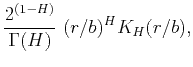
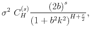
Lord (1954). The statistical autocorrelation
and the energy spectrum
describes a self-affine medium relevant for
geological structures
(Goff and Jordan, 1988; Klimes, 2002; Dolan et al., 1998; Goff and Holliger, 2003; Sato and Fehler, 1998; Holliger and Levander, 1992).
This function was initially derived by von Kármán (1948) while
studying the velocity field in a turbulent fluid and has been used to
describe heterogeneous media (Frankel and Clayton, 1986; Tatarski, 1961). The
Fourier transform of
was given by
Lord (1954). The statistical autocorrelation
and the energy spectrum
 in the Fourier
domain are
in the Fourier
domain are
where
 ,
,  is the modified Bessel function
of the second kind with order
is the modified Bessel function
of the second kind with order  , and
, and  is the Gamma function.
Parameters describing the heterogeneities are characteristic distance
is the Gamma function.
Parameters describing the heterogeneities are characteristic distance  ,
below which the distribution is fractal,
and exponent , characterizing the roughness of the medium.
We use the energy spectrum in equation 7 with
,
below which the distribution is fractal,
and exponent , characterizing the roughness of the medium.
We use the energy spectrum in equation 7 with  to analyze sonic logs
and with
to analyze sonic logs
and with  to predict 3D scattering attenuation.
Subsections
|
|
|
|
| Fractal heterogeneities in sonic logs
and low-frequency scattering attenuation | |
|
Next: Fractal statistics
Up: Browaeys & Fomel: Fractals
Previous: Introduction
2013-03-02