|
|
|
|
Seismic data interpolation beyond aliasing using regularized nonstationary autoregression |
|
|---|
|
sean,sean2
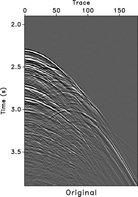
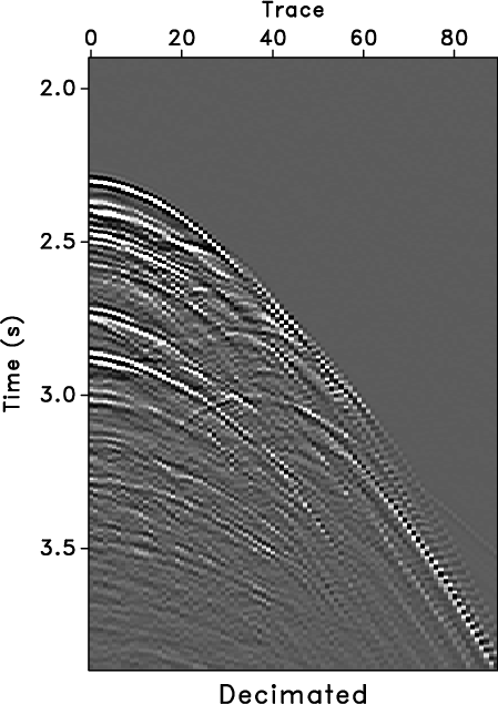
Figure 5. A 2-D marine shot gather. Original input (a) and input subsampled by a factor of 2 (b). |
|
|
|
|---|
|
samiss,serr
Figure 6. Shot gather after trace interpolation (adaptive PEF with 15 |
|
|
|
|---|
|
win,win2
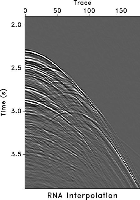
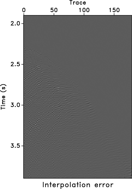
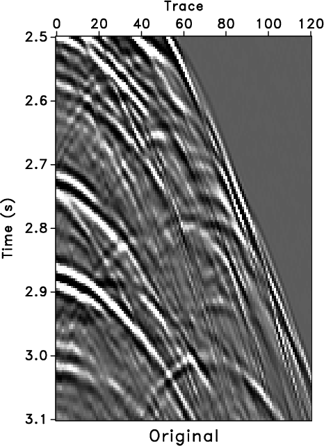
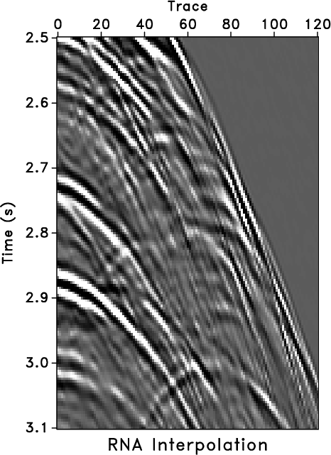
Figure 7. Close-up comparison of original data (a) and interpolated result by RNA (b). |
|
|
|
|---|
|
sfcoe,smcoe
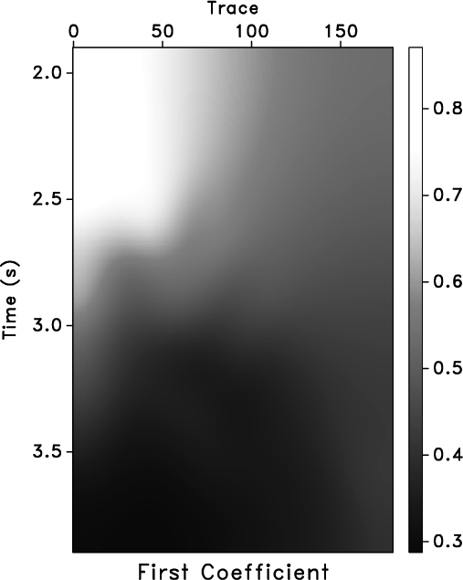
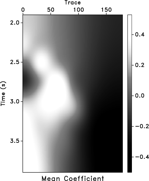
Figure 8. Adaptive PEF coefficients. First coefficient |
|
|
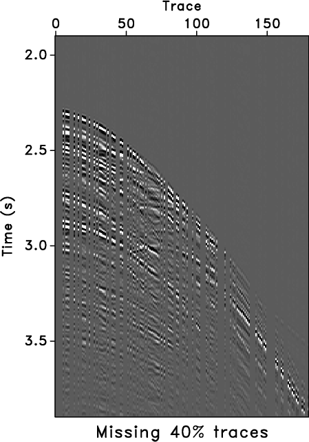
For a missing-trace interpolation test
(Figure 9a), we removed 40% of randomly selected
traces from the input data
(Figure 5a). Furthermore, the first five traces
were also removed to simulate traces missing at near offset. The
adaptive PEF can only use a small number of coefficients in the
spatial direction because of a small number of fitting equations
(where the adaptive PEF lies entirely on known data). However, it also
limits the ability of the proposed method to interpolate dipping
events. We used a nonstationary PEF with 4 (time) ![]() 3 (space)
coefficients for each sample and a 50-sample (time)
3 (space)
coefficients for each sample and a 50-sample (time) ![]() 10-sample
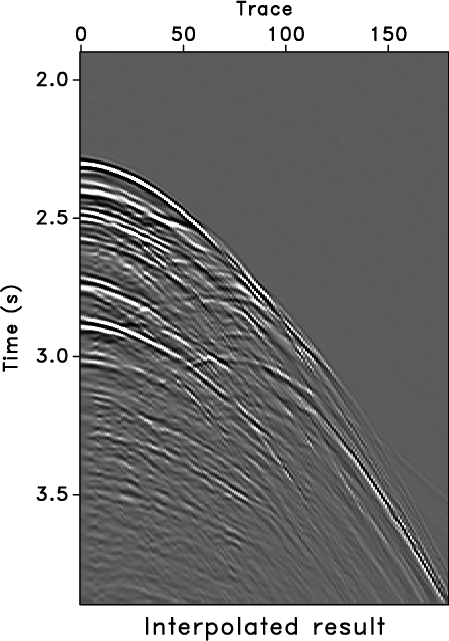
(space) smoothing radius to handle the missing trace recovery. The
result is shown in Figure 9b. By comparing the
results with the original input (Figure 5a), the
missing traces are interpolated reasonably well except for weaker
amplitude of the steeply dipping events.
10-sample
(space) smoothing radius to handle the missing trace recovery. The
result is shown in Figure 9b. By comparing the
results with the original input (Figure 5a), the
missing traces are interpolated reasonably well except for weaker
amplitude of the steeply dipping events.
|
|---|
|
zero,ramiss
Figure 9. Field data with 40% randomly missing traces (a), and reconstructed data using RNA (b). |
|
|
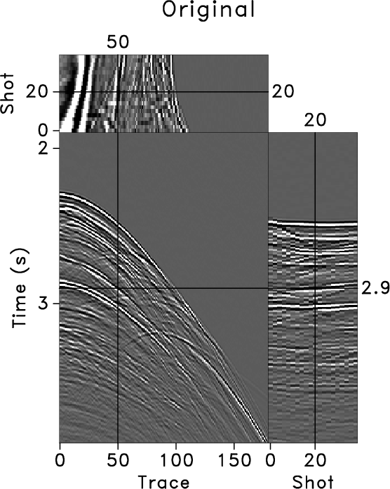
An extension of the method to 3-D is straightforward and follows a
two-step least-squares method with 3-D adaptive PEF
estimation. We use a set of shot gathers as the input data volume to
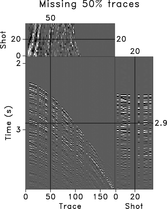
further test our method (Figure 10a). We removed
50% of randomly selected traces and five near offset traces for all
shots (Figure 10b). For comparison, we used
PWD to recover the missing traces
(Figure 11a). The PWD method produces
a reasonable result after carefully estimating dip information, but
the interpolated error is slightly larger in the diffraction
locations. (Figure 11b). The additional
direction provided more information for interpolation but also
increased the number of zeros in the mask operator ![]() , which
constrains enough fitting equations in equation 13. To use
the available fitting equations for adaptive PEF estimation, we chose
a smaller number of coefficients in the spatial direction. The
proposed method is able to handle conflicting dips, although it does
not appear to improve the dipping-event recovery compared to the 2-D
case. This characteristic partly limits the application of RNA in 3-D
case. We used a 3-D nonstationary PEF with 4 (time)
, which
constrains enough fitting equations in equation 13. To use
the available fitting equations for adaptive PEF estimation, we chose
a smaller number of coefficients in the spatial direction. The
proposed method is able to handle conflicting dips, although it does
not appear to improve the dipping-event recovery compared to the 2-D
case. This characteristic partly limits the application of RNA in 3-D
case. We used a 3-D nonstationary PEF with 4 (time) ![]() 2
(space)
2
(space) ![]() 2 (space) coefficients for each sample and a
50-sample (time)
2 (space) coefficients for each sample and a
50-sample (time) ![]() 10-sample (space)
10-sample (space) ![]() 10-sample (space)
smoothing radius was selected. Similar to the result in the 2-D
example, Figure 11c shows the
interpolation result, in which only steeply-dipping low-amplitude
diffraction events with are lost
(Figure 11d).
10-sample (space)
smoothing radius was selected. Similar to the result in the 2-D
example, Figure 11c shows the
interpolation result, in which only steeply-dipping low-amplitude
diffraction events with are lost
(Figure 11d).
|
|---|
|
sean3,zero3
Figure 10. A 3-D field data volume (a) and data with 50% randomly missing traces (b). |
|
|


|
|---|
|
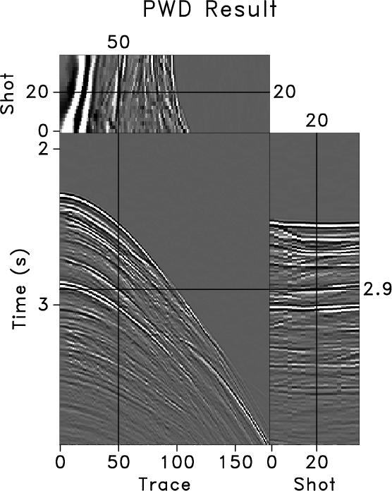
miss3,diff3,amiss3,adiff3
Figure 11. Reconstructed data volume using 3-D plane-wave destruction (a), difference between original input (Figure 10a) and interpolated result (Figure 11a), reconstructed data volume using 3-D regularized nonstationary autogression (c), and difference between original input (Figure 10a) and interpolated result (Figure 11c) (d). |
|
|
|
|
|
|
Seismic data interpolation beyond aliasing using regularized nonstationary autoregression |