 |
 |
 |
 | Signal and noise separation in prestack seismic data using velocity-dependent seislet transform |  |
![[pdf]](icons/pdf.png) |
Next: Synthetic Data Examples
Up: Theory
Previous: VD-slope pattern for pegleg
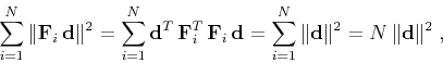
Once the VD-seislet transform is defined, it can be applied to analyze
signals composed of multiple wavefields, e.g., primaries and multiples
of different orders. If a range of slopes are chosen and a VD-seislet
transform is constructed for each of them, then all the transforms
together will constitute an overcomplete
representation. Mathematically, if  is the VD-seislet
transform for the
is the VD-seislet
transform for the  th slope pattern (corresponding to primaries or
pegleg multiples of different orders), then, for any data vector
th slope pattern (corresponding to primaries or
pegleg multiples of different orders), then, for any data vector
 ,
,
 |
(11) |
which means that all transforms taken together constitute a
tight frame with constant  (Mallat, 2009).
Because of its overcompleteness, a frame representation for a given
signal is not unique. In order to assure that different wavefield
components do not leak into other parts of the frame, it is
advantageous to employ sparsity-promoting inversion
(Fomel and Liu, 2010). We use a nonlinear shaping-regularization scheme
(Fomel, 2008) and define sparse decomposition as an iterative
thresholding process (Daubechies et al., 2004)
where  are coefficients of the seislet
frame at
are coefficients of the seislet
frame at  th iteration,
 is an auxiliary
quantity,
is an auxiliary
quantity,  is a soft thresholding operator,
  and
and  are frame construction and deconstruction operators
The iteration in equations 12 and 13
starts with
 and
and
 and is related to the
linearized Bregman iteration (Cai et al., 2009), which converges to the
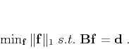
solution of the constrained minimization problem:
and is related to the
linearized Bregman iteration (Cai et al., 2009), which converges to the
solution of the constrained minimization problem:
 |
(18) |
Separated wavefield can be calculated by
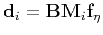 , where
  is
iteration number, masking operator
is
iteration number, masking operator  is a diagonal matrix
as
is a diagonal matrix
as
![\begin{displaymath}
\mathbf{M}_i =
\left[\begin{array}{ccccccc}
\mathbf{0} ...
...ts & \cdots & \mathbf{0}\\
\end{array}\right]_{N\times N}\;,
\end{displaymath}](img85.png) |
(19) |
and  corresponds to
the signal of interest (e.g., primaries or multiples of selected
order). We calculate all patterns for primaries and
multiples, and then apply sparse decomposition (equations 12 and
13) to separate primaries from multiples. In practice,
a small number of iterations is usually sufficient for convergence and
for achieving both model sparseness and data recovery.
corresponds to
the signal of interest (e.g., primaries or multiples of selected
order). We calculate all patterns for primaries and
multiples, and then apply sparse decomposition (equations 12 and
13) to separate primaries from multiples. In practice,
a small number of iterations is usually sufficient for convergence and
for achieving both model sparseness and data recovery.
|
|
|
|
| Signal and noise separation in prestack seismic data using velocity-dependent seislet transform | |
|
Next: Synthetic Data Examples
Up: Theory
Previous: VD-slope pattern for pegleg
2015-10-24
![$\displaystyle \left[\begin{array}{cccc}\mathbf{F}_1 &\mathbf{F}_2 &
\cdots &\mathbf{F}_N\end{array}\right]^T\;,$](img72.png)