|
|
|
|
Seismic data interpolation without iteration using |
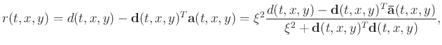
The SPF error ![]() can be expressed as follows:
can be expressed as follows:
When a missing data is encountered, ![]() can be assigned as
zero, and equation 9 can be reduced to:
can be assigned as
zero, and equation 9 can be reduced to:
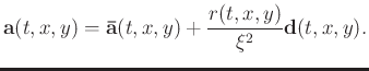
To use the available data for SPF estimation, we designed a 3D
![]() -
-![]() -
-![]() non-causal in space SPF shown in
Figure 1a, the light-gray grids represent
prediction samples and the dark-gray ones exhibit target positions,
whereas white grids represent unused samples. Non-causal in space SPF
utilizes more adjoining traces around the target traces to predict
signals, therefore, it can provide more accurate interpolated results
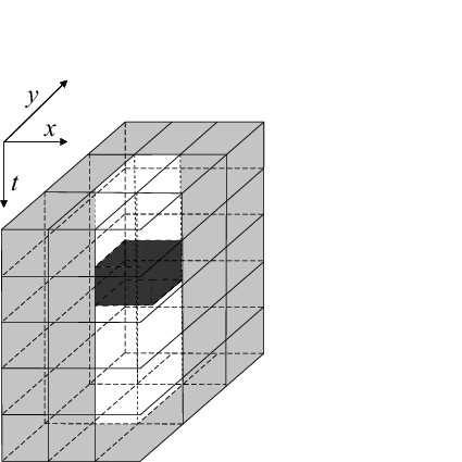
than the causal in space version. The interpolation steps in the 2D
case are illustrated schematically in
Figure 1b. The black and white circles
represent the known data and the missing data,
respectively. Meanwhile, the dotted part is the prior non-causal SPF
position, and dark-grey triangle is the target position. When the
target position is known, the SPF coefficients
non-causal in space SPF shown in
Figure 1a, the light-gray grids represent
prediction samples and the dark-gray ones exhibit target positions,
whereas white grids represent unused samples. Non-causal in space SPF
utilizes more adjoining traces around the target traces to predict
signals, therefore, it can provide more accurate interpolated results
than the causal in space version. The interpolation steps in the 2D
case are illustrated schematically in
Figure 1b. The black and white circles
represent the known data and the missing data,
respectively. Meanwhile, the dotted part is the prior non-causal SPF
position, and dark-grey triangle is the target position. When the
target position is known, the SPF coefficients
![]() can
be obtained from equation 9. In streaming computation, we
can use the time or space axis as the interpolation direction. The
light-gray area in Figure 1b is the position
where the SPF moves next, and the target trace becomes missing
data. Further, spatial gaps are reconstructed according to
equation 12 and 13. Note that the prior filter
coefficients are required in this calculation. If the first target
position is missing trace, e.g., marine data with near-offset missing,
one may use the mirror data to initialize the coefficients of SPF in
the space directions.
can
be obtained from equation 9. In streaming computation, we
can use the time or space axis as the interpolation direction. The
light-gray area in Figure 1b is the position
where the SPF moves next, and the target trace becomes missing
data. Further, spatial gaps are reconstructed according to
equation 12 and 13. Note that the prior filter
coefficients are required in this calculation. If the first target
position is missing trace, e.g., marine data with near-offset missing,
one may use the mirror data to initialize the coefficients of SPF in
the space directions.
We also interpolated the results in the forward and backward spatial
directions; adding the two results
![]() can
reduce the interpolated error caused by the directional properties of
the streaming computation, where
can
reduce the interpolated error caused by the directional properties of
the streaming computation, where ![]() is the forward
interpolated result and
is the forward
interpolated result and ![]() is the backward one. The proposed
method uses local varying smoothness of SPF to characterize time-space
variation of nonstationary data, the analytical calculation of the
inverse matrix in equation 6 avoids iteration, which results
in superior computational speed. Table 1 compares the computational
cost between 3D Fourier POCS (Abma and Kabir, 2006) and the 3D
is the backward one. The proposed
method uses local varying smoothness of SPF to characterize time-space
variation of nonstationary data, the analytical calculation of the
inverse matrix in equation 6 avoids iteration, which results
in superior computational speed. Table 1 compares the computational
cost between 3D Fourier POCS (Abma and Kabir, 2006) and the 3D ![]() -
-![]() -
-![]() SPF. The proposed method occupies less computational resources by
reducing the cost to a single convolution.
SPF. The proposed method occupies less computational resources by
reducing the cost to a single convolution.
| Method | Cost | Filter storage |
| 3D Fourier POCS |
|
|
|
|
|
|
|---|
|
filter3d,filter2d
Figure 1. (a) Schematic illustration of a 3D non-causal in space SPF and (b) interpolation process. |
|
|
|
|
|
|
Seismic data interpolation without iteration using |