|
 |
 |
 | Seismic data interpolation without iteration using  -
- -
- streaming prediction filter with varying smoothness
 |  |
![[pdf]](icons/pdf.png) |
Next: Step 2: Data interpolation
Up: Theory
Previous: Theory
Linear events with different constant dips can be predicted by a PF or
an autoregression operator in the time-space domain, which is
calculated to minimize the energy of the prediction error. Consider a
3D
-
-
PF  to predict a given centered sample
 of data:
 |
(1) |
where
 represents the translation of
with
time shifts
represents the translation of
with
time shifts  and space shifts
  and
and  , nonstationary filter
coefficients
, nonstationary filter
coefficients
 change with time and space axes, and
 ,
,  , and
, and  control the lengths of the filter along
,
,
and
-axes, respectively.
control the lengths of the filter along
,
,
and
-axes, respectively.
In linear algebra notation, the filter coefficients
are
determined by minimizing the underdetermined least-squares problem:
 |
(2) |
where
 represents the vector of filter coefficients
and
represents the vector of filter coefficients
and
 represents the vector of data translations
. For nonstationary situations, we can use
different regularization term to constrain equation 2, such
as global smoothness (Liu and Fomel, 2011). Sacchi and Naghizadeh (2009) introduced a
local smoothness constraint to calculate the adaptive prediction
filter. Fomel and Claerbout (2016) proposed the same constraint and solved the
algebraic problem analytically with streaming computation, which
demonstrated the same results as Sacchi and Naghizadeh's method. The
local constraint is that the new filter
represents the vector of data translations
. For nonstationary situations, we can use
different regularization term to constrain equation 2, such
as global smoothness (Liu and Fomel, 2011). Sacchi and Naghizadeh (2009) introduced a
local smoothness constraint to calculate the adaptive prediction
filter. Fomel and Claerbout (2016) proposed the same constraint and solved the
algebraic problem analytically with streaming computation, which
demonstrated the same results as Sacchi and Naghizadeh's method. The
local constraint is that the new filter
 stays close to
the prior neighboring filter
stays close to
the prior neighboring filter
 ,
,
 , where
  is a scale
parameter. However, the regularization term occasionally fails in the
presence of strong amplitude variation. Thus, we improved the
constraint with varying smoothness. The SPF in the
-
-
domain
was found by solving the least-squares problem:
is a scale
parameter. However, the regularization term occasionally fails in the
presence of strong amplitude variation. Thus, we improved the
constraint with varying smoothness. The SPF in the
-
-
domain
was found by solving the least-squares problem:
 |
(3) |
where
 is the similarity matrix, which controls the
closeness between the adjacent filters. For the design of
, we can use the data value and follow three principles:
is the similarity matrix, which controls the
closeness between the adjacent filters. For the design of
, we can use the data value and follow three principles:
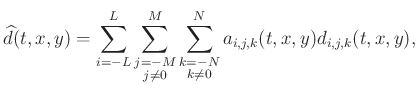
1. Usage of PF to characterize the energy spectra of data; hence, both
the adjacent data and the adjacent PFs are similar based on local
plane wave assumption. Therefore,
should be close to
identity matrix.
2. Data value is not be used alone in the
expression of
; otherwise, the calculation will be
unstable because there exists large number of data with zero value in
the missing seismic data.
3. The variation of data value can
reasonably control the local smoothness of filter coefficients.
In this study, we designed the
based on
the amplitude difference of the smoothed data:
where  is the sale factor and
  represent the
smooth version of data that are less affected by random noise, e.g.,
the preprocessed data using Gaussian filter.
represent the
smooth version of data that are less affected by random noise, e.g.,
the preprocessed data using Gaussian filter.
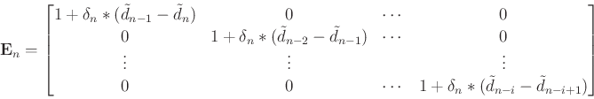
In a 3D case, the regularization term in equation 3 should
include three directions:
 |
(5) |
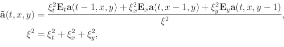
The least-squares solution of equation 3 is:
![$\displaystyle \mathbf{a}(t,x,y)=[\mathbf{d}(t,x,y)\mathbf{d}(t,x,y)^{T}+\xi^2\mathbf{I}]^{-1} [d(t,x,y)\mathbf{d}(t,x,y)+\xi^2\mathbf{\tilde{a}}(t,x,y)],$](img45.png) |
(6) |
where
and
 is the identity matrix. The regularization terms
 should have the same order of magnitude as the data. From
equation 7, we can consider
should have the same order of magnitude as the data. From
equation 7, we can consider
 as a
whole term, which provides an adaptive smoothness for the
nonstationary PF.
as a
whole term, which provides an adaptive smoothness for the
nonstationary PF.
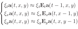
In equation 5, a stable update of SPF requires that the
adjacent filter coefficients have the same order of magnitude, and the
stable condition is based on the selection of the parameters
and
. We can calculate the difference between the
maximum and minimum values in the data, and
is selected as
the reciprocal of this difference to guarantee that
may
be close to the identity matrix. Meanwhile, the parameter
should be chosen to the constant value between the minimum and maximum
values of the data according to the smoothness level of the
regularization.
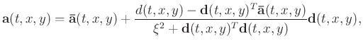
The inverse matrix in equation 6 can be directly calculated
without iterative conjugate-gradient method. Sherman-Morrison formula
(Hager, 1989) provided an analytic solution for the inverse of a
special matrix like
 , where matrix
 is a column vector and matrix
 is a row
vector. If
is a row
vector. If
 and
and
 are invertible, the
inverse matrix results in:
are invertible, the
inverse matrix results in:
 |
(8) |
In this paper,
 ,
,
 and
and
 in equation 8. After
algebraic simplification, the filter coefficients arrive at the explicit solution as given below:
in equation 8. After
algebraic simplification, the filter coefficients arrive at the explicit solution as given below:
 |
(9) |
|
|
|
|
| Seismic data interpolation without iteration using
-
-
streaming prediction filter with varying smoothness | |
|
Next: Step 2: Data interpolation
Up: Theory
Previous: Theory
2022-04-12